Why Deep Learning for Genomics?
GENE 46100 — Unit 0
2025-03-25
Course Roadmap
| Unit | Topic |
|---|---|
| 0 | MLP, CNN, DNA scoring |
| 1 | Transformers & Genomic GPT |
| 2 | Enformer & Borzoi |
| 3 | Applications |
Tools we’ll use:
- Python + PyTorch
- Google Colab (GPU)
- Weights & Biases
By the end: You’ll understand how state-of-the-art models predict gene expression from DNA sequence
What Can Deep Learning Do in Genomics?
- Predict TF binding from DNA sequence alone
- Score regulatory variants without experiments
- Predict gene expression from 200kb of sequence (Enformer)
- Generate protein structures (AlphaFold)
- Build DNA language models that learn grammar of the genome
These models learn patterns we didn’t know to look for.
The Starting Point: Linear Models
You already know this from statistics/ML:
\[y = X\beta + \epsilon\]
Closed-form solution: \(\hat{\beta} = (X^TX)^{-1}X^Ty\)
Works great when the relationship is linear.
But what if it’s not?
What If the Truth Is Curved?
Consider: \(y = x^3\)
Linear model:
- Fits best straight line
- Residuals are huge
- Fundamentally wrong model
What we need:
- A model that can learn any shape
- Without us specifying the functional form
- From data alone
You’ll see this exact demo in the hands-on notebook
Gradient Descent: Learning by Iterating
Instead of a closed-form solution, we iteratively improve:
- Start with random parameters
- Compute prediction error (loss)
- Compute gradient: which direction reduces loss?
- Take a small step in that direction
- Repeat
\[\theta_{t+1} = \theta_t - \alpha \nabla L(\theta_t)\]
Why? Because for nonlinear models, there’s no closed-form solution.
Enter the MLP
Multi-Layer Perceptron — the simplest neural network
MLP: The Math
The formula for one hidden layer:
\[y = W_2 \cdot \sigma(W_1 x + b_1) + b_2\]
The activation function \(\sigma\) (e.g., ReLU) is what makes it nonlinear.
Why the Activation Function Matters
Without activation: stacking linear layers is still linear
\[W_2(W_1 x) = (W_2 W_1) x = W'x\]
With ReLU activation: \(\text{ReLU}(x) = \max(0, x)\)
- Each neuron becomes a “hinge”
- Combinations of hinges approximate any curve
- More neurons → better approximation
Universal Approximation Theorem
An MLP with a single hidden layer can approximate any continuous function to arbitrary accuracy, given enough hidden neurons.
What this means for us:
- We don’t need to know the functional form
- The network learns it from data
- We just need enough neurons and enough data
What this doesn’t mean:
- It doesn’t say learning is easy
- It doesn’t say how many neurons you need
- It doesn’t say it will generalize
PyTorch: Automatic Differentiation
The key idea: you define the forward pass, PyTorch computes the gradients
# Define model
model = MLP(input_dim=1, hidden_dim=64, output_dim=1)

# Training loop
for epoch in range(1000):
    y_hat = model(x)          # forward pass
    loss = loss_fn(y_hat, y)  # compute loss
    loss.backward()           # compute gradients (automatic!)
    optimizer.step()          # update parameters
    optimizer.zero_grad()     # reset gradients
You’ll implement this in the hands-on notebook
The Training Loop — Visually
                    ┌─────────────┐
                    │  Input Data │
                    └──────┬──────┘
                           ▼
                    ┌─────────────┐
              ┌────▶│ Forward Pass│
              │     └──────┬──────┘
              │            ▼
              │     ┌─────────────┐
              │     │ Compute Loss│
              │     └──────┬──────┘
              │            ▼
              │     ┌─────────────┐
              │     │  Backward   │ ← PyTorch does this
              │     │  (Gradients)│
              │     └──────┬──────┘
              │            ▼
              │     ┌─────────────┐
              └─────│Update Params│
                    └─────────────┘
DNA as Data: One-Hot Encoding
How do we feed DNA to a neural network?
Sequence:  A  T  G  C  G  T  A

           A  T  G  C
     1:  [ 1  0  0  0 ]  ← A
     2:  [ 0  1  0  0 ]  ← T
     3:  [ 0  0  1  0 ]  ← G
     4:  [ 0  0  0  1 ]  ← C
     5:  [ 0  0  1  0 ]  ← G
     6:  [ 0  1  0  0 ]  ← T
     7:  [ 1  0  0  0 ]  ← A
Shape: (sequence_length, 4)
Each base → a 4-dimensional unit vector. No ordinal relationship imposed.
From DNA to Prediction
DNA sequence          One-hot matrix       Neural network      Prediction

ATGCGTAACG...  →  ┌─────────────┐   →   ┌──────────┐   →   binding score
                  │ 1 0 0 0     │       │  MLP or  │       expression level
                  │ 0 1 0 0     │       │   CNN    │       variant effect
                  │ 0 0 1 0     │       │          │       ...
                  │ 0 0 0 1     │       └──────────┘
                  │ ...         │
                  └─────────────┘
This is the core pattern of the entire course.
Every model we study takes DNA sequence as input and predicts a biological output.
MLP vs CNN: A Preview
MLP (this week)
- Flatten DNA → single vector
- Every input connected to every neuron
- No concept of “position”
- Good for learning the basics
CNN (next week)
- Preserve 2D structure
- Sliding window = motif scanner
- Learned filters ≈ PWMs
- The workhorse of genomic DL
Key question CNN answers: Is there a motif anywhere in this sequence?
Why CNNs Work for DNA
A CNN filter sliding over one-hot DNA is mathematically equivalent to scoring with a Position Weight Matrix (PWM)
Filter:  [weights for A, T, G, C] × filter_length

   = a learned PWM!
But better:
- Learns the motifs from data (no database needed)
- Stacks of filters capture combinations of motifs
- Multiple layers capture hierarchical patterns
Erin Wilson’s DNA scoring notebook makes this beautifully concrete
Unit 0 Plan: Weeks 1–3
| Session | Topic | Notebook |
|---|---|---|
| Week 1a | Setup, intro | (this lecture) |
| Week 1b | Linear → MLP in PyTorch | hands-on-introduction_to_deep_learning.ipynb |
| Week 2 | CNN for DNA scoring | updated-basic_DNA_tutorial.ipynb |
| Week 3a | TF binding project | tf-binding-prediction-starter.ipynb |
| Week 3b | Hyperparameter tuning | tf-binding-wandb.ipynb |
What’s Coming Next
Unit 1: Transformers & GPT
- Attention mechanism
- Karpathy’s nanoGPT
- Train a DNA language model
- Fine-tune for promoter prediction
Unit 2: Enformer & Borzoi
- Predict epigenome from 200kb DNA
- Variant effect prediction
- Connection to GWAS/PrediXcan
The arc: MLP → CNN → Transformer → Genomic foundation models
Getting Started
Environment: Google Colab (GPU provided, no local setup needed)
First notebook: hands-on-introduction_to_deep_learning.ipynb
You will:
- Fit a linear model with gradient descent
- See it fail on nonlinear data
- Build an MLP that succeeds
- Visualize the learning curve
Resources
Videos:
- 3Blue1Brown: Neural Networks — beautiful visual intuition
- Karpathy: Building GPT from scratch — we’ll use this in Unit 1
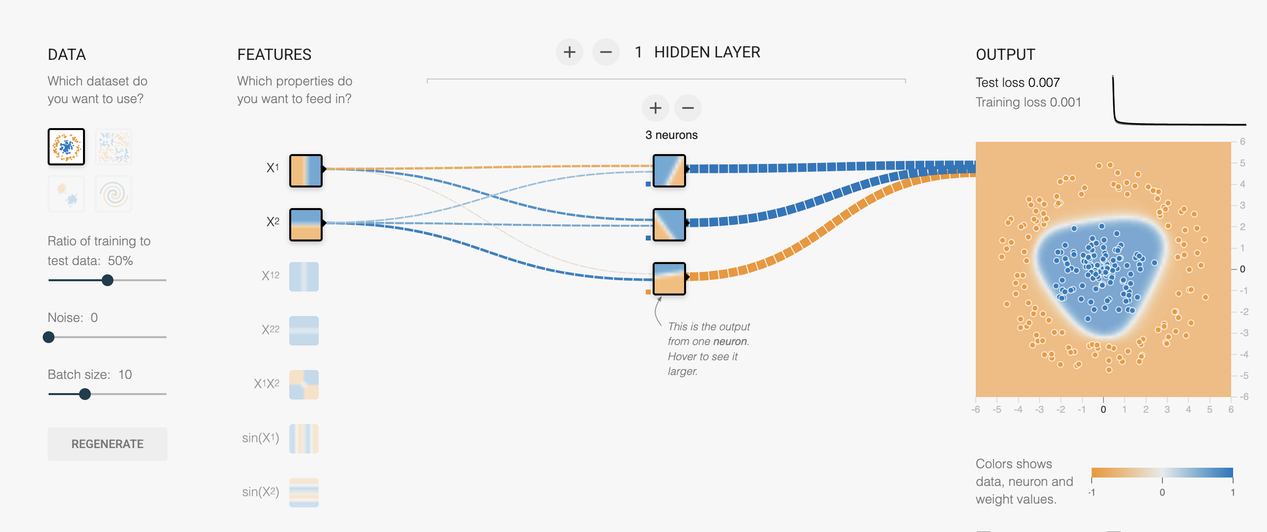
Interactive:
- playground.hakyimlab.org — experiment with MLP architecture interactively
Papers (optional):
- Avsec et al. 2021 — Enformer
- Linder et al. 2023 — Borzoi
Questions?
GENE 46100 · Deep Learning in Genomics