if False:
    %pip install seaborn matplotlib logomaker

if False: # these were installed with the intro notebook
    %pip install scikit-learn plotnine tqdm pandas
    %pip install numpy ## gets installed with scikit-learn
    %pip install tqdm
    %pip install torch
    %pip install torchvision torchmetrics
Updated - DNA score prediction with Pytorch
gene46100
notebook
created by Erin Wilson. Downloaded from here.
Some edits by Haky Im and Ran Blekhman for the deep learning in genomics gene46100 course.
- changed names of functions to improve readability
- adapted for compatibility with Apple Silicon (M1/M2/M3) MacBooks using MPS
- Using float32 instead of float64 (MPS doesn’t support double precision)
- Setting device to ‘mps’ when available
- Ensuring tensor data types are compatible with Metal Performance Shaders (MPS)
- conda installation steps removed, issues with versions and pytorch mps compatibility
- added questions
Environment Setup
We use minimal conda environment gene41600 (instructions here) and install python packages with %pip instead due to fewer version conflicts, especially for M-series Macs. See installation steps below.
Tutorial Overview
This tutorial shows an example of a Pytorch framework that can use raw DNA sequences as input, feed these into a neural network model, and predict a quantitative label directly from the sequence.
- Generate synthetic DNA data
- Prepare data for Pytorch training
- Define Pytorch models
- Define training loop functions
- Train the models
- Check model predictions on test set
- Visualize convolutional filters
- Conclusion
It assumes the reader is already familiar with ML concepts like: * What is a neural network? * Basics of a convolutional neural network (CNN) * Model training over epochs * Splitting data into train/val/test sets * Loss functions and comparing train vs val loss curves
It also assumes some familiarity with biological concepts like: * DNA nucleotides * What is a regulatory motif? * visualizing DNA motifs
import necessary modules
from collections import defaultdict
from itertools import product
import matplotlib.pyplot as plt
import numpy as np
import pandas as pd
import random
import torch
from torch import nn
import torch.nn.functional as F


if torch.backends.mps.is_available():
    torch.set_default_dtype(torch.float32)
    print("Set default to float32 for MPS compatibility")
Set default to float32 for MPS compatibilityset seeds for reproduciblity across runs
# Set a random seed in a bunch of different places
def set_seed(seed: int = 42) -> None:
    np.random.seed(seed)
    random.seed(seed)
    torch.manual_seed(seed)

    if torch.backends.mps.is_available():
        # For MacBooks with Apple Silicon
        torch.mps.manual_seed(seed)
    elif torch.cuda.is_available():
        # For CUDA GPUs
        torch.cuda.manual_seed(seed)
        torch.backends.cudnn.deterministic = True
        torch.backends.cudnn.benchmark = False
    print(f"Random seed set as {seed}")

set_seed(17)
Random seed set as 17define GPU device
Are you working on a GPU? If so, you can put your data/models on DEVICE (and have to do so explicity)! If not, you can probably remove all instances of foo.to(DEVICE) and it should still work fine on a CPU.
DEVICE = torch.device('mps' if torch.backends.mps.is_available()
                     else 'cuda' if torch.cuda.is_available()
                     else 'cpu')
DEVICEdevice(type='mps')## 1. Generate synthetic DNA data
Usually scientists might be interested in predicting something like a binding score, an expression strength, or classifying a TF binding event. But here, we are going to keep it simple: the goal in this tutorial is to observe if a deep learning model can learn to detect a very small, simple pattern in a DNA sequence and score it appropriately (again, just a practice task to convince ourselves that we have actually set up the Pytorch pieces correctly such that it can learn from input that looks like a DNA sequence).
So arbitrarily, let’s say that given an 8-mer DNA sequence, we will score it based on the following rules: * A = +20 points * C = +17 points * G = +14 points * T = +11 points
For every 8-mer, let’s sum up its total points based on the nucleotides in its sequence, then take the average. For example,
AAAAAAAAwould score20.0- (
mean(20 + 20 + 20 + 20 + 20 + 20 + 20 + 20) = 20.0)
- (
ACAAAAAAwould score19.625- (
mean(20 + 17 + 20 + 20 + 20 + 20 + 20 + 20) = 19.625)
- (
These values for the nucleotides are arbitrary - there’s no real biology here! It’s just a way to assign sequences a score for the purposes of our Pytorch practice.
However, since many recent papers use methods like CNNs to automatically detect “motifs,” or short patterns in the DNA that can activate or repress a biological response, let’s add one more piece to our scoring system. To simulate something like motifs influencing gene expression, let’s say a given sequence gets a +10 bump if TAT appears anywhere in the 8-mer, and a -10 bump if it has a GCG in it. Again, these motifs don’t mean anything in real life, they are just a mechanism for simulating a really simple activation or repression effect.
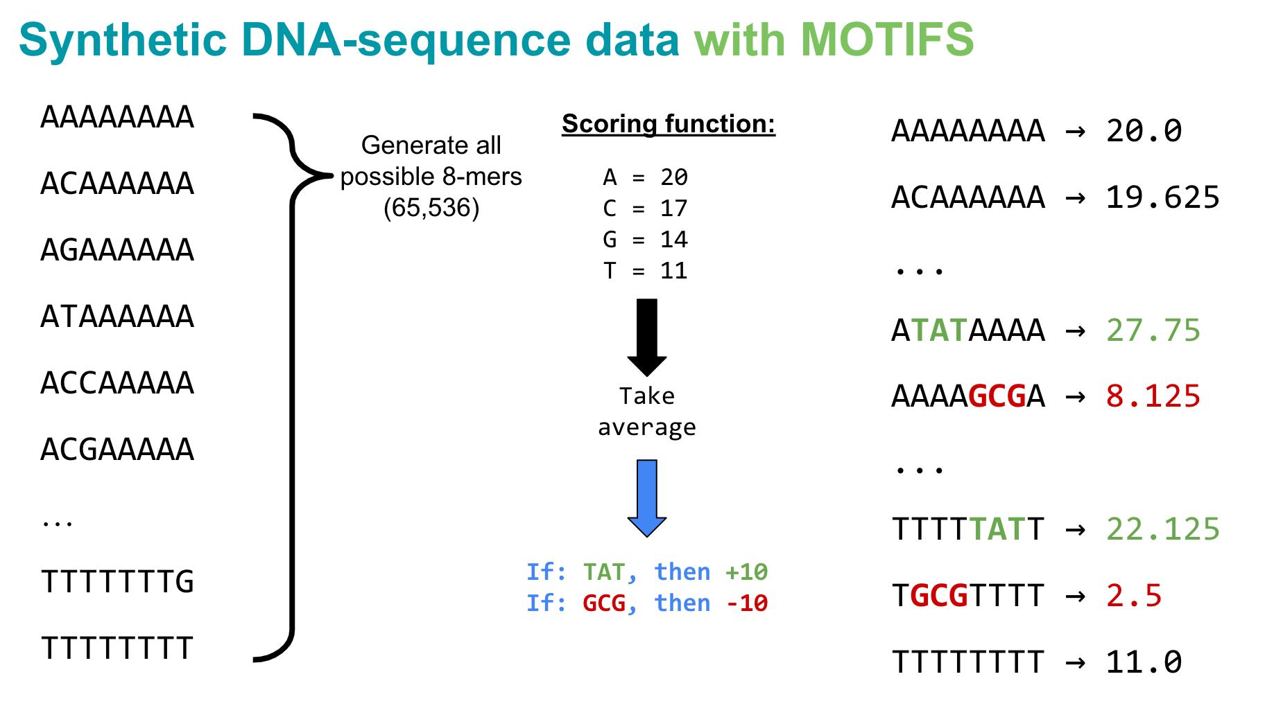
So let’s implement this basic scoring function!
# define function for generating all k-mers of length k
def kmers(k):
    '''Generate a list of all k-mers for a given k'''

    return [''.join(x) for x in product(['A','C','G','T'], repeat=k)]
generate all 8-mers
# generate all 8-mers
seqs8 = kmers(8)
print('Total 8mers:',len(seqs8))
Total 8mers: 65536define scoring function for the DNA sequences
# define score_dict
score_dict = {
    'A':20,
    'C':17,
    'G':14,
    'T':11
}
# define function for scoring sequences
def score_seqs_motif(seqs):
    '''
    Calculate the scores for a list of sequences based on
    the above score_dict
    '''
    data = []
    for seq in seqs:
        # get the average score by nucleotide
        score = np.mean([score_dict[base] for base in seq],dtype=np.float32)

        # give a + or - bump if this k-mer has a specific motif
        if 'TAT' in seq:
            score += 10
        if 'GCG' in seq:
            score -= 10
        data.append([seq,score])

    df = pd.DataFrame(data, columns=['seq','score'])
    return df
mer8 = score_seqs_motif(seqs8)
mer8.head()| seq | score | |
|---|---|---|
| 0 | AAAAAAAA | 20.000 |
| 1 | AAAAAAAC | 19.625 |
| 2 | AAAAAAAG | 19.250 |
| 3 | AAAAAAAT | 18.875 |
| 4 | AAAAAACA | 19.625 |
Spot check scores of a couple seqs with motifs:
mer8[mer8['seq'].isin(['TGCGTTTT','CCCCCTAT'])]| seq | score | |
|---|---|---|
| 21875 | CCCCCTAT | 25.875 |
| 59135 | TGCGTTTT | 2.500 |
plot distribution of motif scores
plt.hist(mer8['score'].values,bins=20)
plt.title("8-mer with Motifs score distribution")
plt.xlabel("seq score",fontsize=14)
plt.ylabel("count",fontsize=14)
plt.show()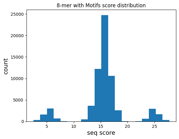
As expected, the distribution of scores across all 8-mers has 3 groups: * No motif (centered around ~15) * contains TAT (~25) * contains GCG (~5)
Question 1
Modify the scoring function to create a more complex pattern. Instead of giving fixed bonuses for “TAT” and “GCG”, implement a position-dependent scoring where a motif gets a higher bonus if it appears at the beginning of the sequence compared to the end. How does this change the distribution of scores?
Next, we want to train a model to predict this score by from the DNA sequence
## 2. Prepare data for Pytorch training
For neural networks to make predictions, you have to give it your input as a matrix of numbers. For example, to classify images by whether or not they contain a cat, a network “sees” the image as a matrix of pixel values and learns relevant patterns in the relative arrangement of pixels (e.g. patterns that correspond to cat ears, or a nose with whiskers).
We similarly need to turn our DNA sequences (strings of ACGTs) into a matrix of numbers. So how do we pretend our DNA is a cat?
One common strategy is to one-hot encode the DNA: treat each nucleotide as a vector of length 4, where 3 positions are 0 and one position is a 1, depending on the nucleotide.
turn DNA sequences into numbers with one hot encoding
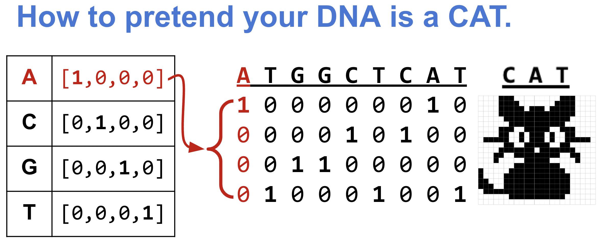
This one-hot encoding has the nice property that it makes your DNA appear like how a computer sees a picture of a cat!
def one_hot_encode(seq):
    """
    Given a DNA sequence, return its one-hot encoding
    """
    # Make sure seq has only allowed bases
    allowed = set("ACTGN")
    if not set(seq).issubset(allowed):
        invalid = set(seq) - allowed
        raise ValueError(f"Sequence contains chars not in allowed DNA alphabet (ACGTN): {invalid}")

    # Dictionary returning one-hot encoding for each nucleotide
    nuc_d = {'A':[1.0,0.0,0.0,0.0],
             'C':[0.0,1.0,0.0,0.0],
             'G':[0.0,0.0,1.0,0.0],
             'T':[0.0,0.0,0.0,1.0],
             'N':[0.0,0.0,0.0,0.0]}

    # Create array from nucleotide sequence
    vec=np.array([nuc_d[x] for x in seq], dtype=np.float32)

    return vec
# one hot encoding of 8 As
a8 = one_hot_encode("AAAAAAAA")
print("AAAAAA:\n",a8)
AAAAAA:
 [[1. 0. 0. 0.]
 [1. 0. 0. 0.]
 [1. 0. 0. 0.]
 [1. 0. 0. 0.]
 [1. 0. 0. 0.]
 [1. 0. 0. 0.]
 [1. 0. 0. 0.]
 [1. 0. 0. 0.]]
# one hot encoding of another DNA
s = one_hot_encode("AGGTACCT")
print("AGGTACC:\n",s)
print("shape:",s.shape)AGGTACC:
[[1. 0. 0. 0.]
[0. 0. 1. 0.]
[0. 0. 1. 0.]
[0. 0. 0. 1.]
[1. 0. 0. 0.]
[0. 1. 0. 0.]
[0. 1. 0. 0.]
[0. 0. 0. 1.]]
shape: (8, 4)split data into train, validation, and test
Data are typically split into training, validation, and test sets. This helps avoid overfitting and achieve better generalization to new data.
- Training set (e.g. 70% of the data)
- used to train the model
- model learns patterns from this data
- analogy: studying for an exam
- Validation or tuning set (e.g. 15% of the data)
- used to tune hypterparameters
- helps prevent overfitting
- analogy: pratice problems while studying
- Test set or held out set (e.g. 15% of the data)
- used only to evaluate final model performance
- never used during training or tuning
- analogy: actual exam
Note: in this tutorial, that uses the quick_split function defined here splits the data into 20% for the test set, 80% of the remaining 80% as the training set (i.e. 64% of the total) and 20% of the non test sets as validation (i.e. 16%).
define quick splitting function
# define function for splitting data
def quick_split(df, split_frac=0.8, verbose=False):
    '''
    Given a df of samples, randomly split indices between
    train and test at the desired fraction
    '''
    cols = df.columns # original columns, use to clean up reindexed cols
    df = df.reset_index()

    # shuffle indices
    idxs = list(range(df.shape[0]))
    random.shuffle(idxs)

    # split shuffled index list by split_frac
    split = int(len(idxs)*split_frac)
    train_idxs = idxs[:split]
    test_idxs = idxs[split:]

    # split dfs and return
    train_df = df[df.index.isin(train_idxs)]
    test_df = df[df.index.isin(test_idxs)]

    return train_df[cols], test_df[cols]
split data into train, validation, and test sets
# split data into train, validation, and test
full_train_df, test_df = quick_split(mer8)
train_df, val_df = quick_split(full_train_df)

print("Train:", train_df.shape)
print("Val:", val_df.shape)
print("Test:", test_df.shape)

train_df.head()
Train: (41942, 2)
Val: (10486, 2)
Test: (13108, 2)| seq | score | |
|---|---|---|
| 0 | AAAAAAAA | 20.000 |
| 1 | AAAAAAAC | 19.625 |
| 2 | AAAAAAAG | 19.250 |
| 3 | AAAAAAAT | 18.875 |
| 4 | AAAAAACC | 19.250 |
plot distribution of train, validation, and test data and check that they are similarly distributed
def plot_train_test_hist(train_df, val_df,test_df,bins=20):
    ''' Check distribution of train/test scores, sanity check that its not skewed'''
    plt.hist(train_df['score'].values,bins=bins,label='train',alpha=0.5)
    plt.hist(val_df['score'].values,bins=bins,label='val',alpha=0.75)
    plt.hist(test_df['score'].values,bins=bins,label='test',alpha=0.4)
    plt.legend()
    plt.xlabel("seq score",fontsize=14)
    plt.ylabel("count",fontsize=14)
    plt.show()
With the below histogram, we can confirm that the train, test, and val sets contain example sequences from each bucket of the distribution (each set has some examples with each kind of motif)
plot_train_test_hist(train_df, val_df,test_df)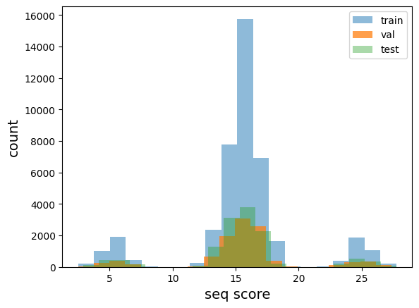
define dataset and dataloader classes
Dataset and DataLoader classes allow efficient data handling in deep learning.
Dataset class allows standardized way to access and preprocess data.
Dataloader handles batching, shuffling, parallel data loading to make it easier to feed the data for training.
You can read more about DataLoader and Dataset objects.
from torch.utils.data import Dataset, DataLoaderdefine one hot encoded dataset class
This class is essential for preparing DNA sequence data for deep learning models, converting the DNA sequences into a numerical format that neural networks can process.
class SeqDatasetOHE(Dataset):
    '''
    Dataset for one-hot-encoded sequences
    '''
    def __init__(self, df, seq_col='seq', target_col='score'):
        # Input: DataFrame with DNA sequences and their scores
        self.seqs = list(df[seq_col].values)  # Get DNA sequences
        self.seq_len = len(self.seqs[0])      # Length of each sequence

        # Convert DNA sequences to one-hot encoding
        self.ohe_seqs = torch.stack([torch.tensor(one_hot_encode(x)) for x in self.seqs])

        # Get target scores
        self.labels = torch.tensor(list(df[target_col].values)).unsqueeze(1)

    def __len__(self): return len(self.seqs)

    def __getitem__(self,idx):
        # Given an index, return a tuple of an X with it's associated Y
        # This is called inside DataLoader
        seq = self.ohe_seqs[idx]
        label = self.labels[idx]

        return seq, label
construct DataLoaders from Datasets.
def build_dataloaders(train_df,
                      test_df,
                      seq_col='seq',
                      target_col='score',
                      batch_size=128,
                      shuffle=True
                     ):
    '''
    Given a train and test df with some batch construction
    details, put them into custom SeqDatasetOHE() objects.
    Give the Datasets to the DataLoaders and return.
    '''

    # create Datasets
    train_ds = SeqDatasetOHE(train_df,seq_col=seq_col,target_col=target_col)
    test_ds = SeqDatasetOHE(test_df,seq_col=seq_col,target_col=target_col)

    # Put DataSets into DataLoaders
    train_dl = DataLoader(train_ds, batch_size=batch_size, shuffle=shuffle)
    test_dl = DataLoader(test_ds, batch_size=batch_size)


    return train_dl,test_dl
train_dl, val_dl = build_dataloaders(train_df, val_df)These dataloaders are now ready to be used in a training loop!
## 3. Define Pytorch models The primary model I was interested in trying was a Convolutional Neural Network, as these have been shown to be useful for learning motifs from genomic data. But as a point of comparison, I included a simple Linear model. Here are some model definitions:
# very simple linear model
class DNA_Linear(nn.Module):
    def __init__(self, seq_len):
        super().__init__()
        self.seq_len = seq_len
        # the 4 is for our one-hot encoded vector length 4!
        self.lin = nn.Linear(4*seq_len, 1)

    def forward(self, xb):
        # reshape to flatten sequence dimension
        xb = xb.view(xb.shape[0],self.seq_len*4)
        # Linear wraps up the weights/bias dot product operations
        out = self.lin(xb)
        return out

## CNN model
class DNA_CNN(nn.Module):
    def __init__(self, seq_len, num_filters=32, kernel_size=3):
        super().__init__()
        self.seq_len = seq_len

        # Define layers individually
        self.conv = nn.Conv1d(4, num_filters, kernel_size=kernel_size)
        self.relu = nn.ReLU(inplace=True)
        self.linear = nn.Linear(num_filters*(seq_len-kernel_size+1), 1)

    def forward(self, xb):
        # reshape view to batch_size x 4channel x seq_len
        xb = xb.permute(0, 2, 1)

        # Apply layers step by step
        x = self.conv(xb)
        x = self.relu(x)
        x = x.flatten(1)  # flatten all dimensions except batch
        out = self.linear(x)
        return out
These aren’t optimized models, just something to start with (again, we’re just practicing connecting the Pytorch tubes in the context of DNA!). * The Linear model tries to predict the score by simply weighting the nucleotides that appears in each position. * The CNN model uses 32 filters of length (kernel_size) 3 to scan across the 8-mer sequences for informative 3-mer patterns.
## 4. Define the training loop functions
The model training process is structured into a series of modular functions, each responsible for a specific part of the workflow. This design improves clarity, reusability, and flexibility when working with different models, optimizers, or loss functions.
The overall structure is as follows:
# Initializes optimizer and loss function if not provided, then trains the model
run_training()

    # Iterates over multiple epochs
    train_loop()

        # Performs one complete pass over the training dataset
        train_epoch()

            # Computes loss and backprops for a single batch
            process_batch()

        # Performs one complete pass over the validation dataset
        val_epoch()

            # Computes loss for a single batch no gradient updates
            process_batch()
# +--------------------------------+
# | Training and fitting functions |
# +--------------------------------+
def process_batch(model, loss_func, xb, yb, opt=None,verbose=False):
'''
Apply loss function to a batch of inputs. If no optimizer
is provided, skip the back prop step.
'''
if verbose:
print('loss batch ****')
print("xb shape:",xb.shape)
print("yb shape:",yb.shape)
print("yb shape:",yb.squeeze(1).shape)
#print("yb",yb)
# get the batch output from the model given your input batch
# ** This is the model's prediction for the y labels! **
xb_out = model(xb.float())
if verbose:
print("model out pre loss", xb_out.shape)
#print('xb_out', xb_out)
print("xb_out:",xb_out.shape)
print("yb:",yb.shape)
print("yb.long:",yb.long().shape)
loss = loss_func(xb_out, yb.float()) # for MSE/regression
# __FOOTNOTE 2__
if opt is not None: # if opt
opt.zero_grad() ## moved zero grad up to make sure it's not accumulating grads from previous batches
loss.backward()
opt.step()
return loss.item(), len(xb)
def train_epoch(model, train_dl, loss_func, device, opt):
'''
Execute 1 set of batched training within an epoch
'''
# Set model to Training mode
model.train()
tl = [] # train losses
ns = [] # batch sizes, n
# loop through train DataLoader
for xb, yb in train_dl:
# put on GPU
xb, yb = xb.to(device),yb.to(device)
# provide opt so backprop happens
t, n = process_batch(model, loss_func, xb, yb, opt=opt)
# collect train loss and batch sizes
tl.append(t)
ns.append(n)
# average the losses over all batches
train_loss = np.sum(np.multiply(tl, ns)) / np.sum(ns)
return train_loss
def val_epoch(model, val_dl, loss_func, device):
'''
Execute 1 set of batched validation within an epoch
'''
# Set model to Evaluation mode
model.eval()
with torch.no_grad():
vl = [] # val losses
ns = [] # batch sizes, n
# loop through validation DataLoader
for xb, yb in val_dl:
# put on GPU
xb, yb = xb.to(device),yb.to(device)
# Do NOT provide opt here, so backprop does not happen
v, n = process_batch(model, loss_func, xb, yb)
# collect val loss and batch sizes
vl.append(v)
ns.append(n)
# average the losses over all batches
val_loss = np.sum(np.multiply(vl, ns)) / np.sum(ns)
return val_loss
def train_loop(epochs, model, loss_func, opt, train_dl, val_dl,device,patience=1000):
'''
Fit the model params to the training data, eval on unseen data.
Loop for a number of epochs and keep train of train and val losses
along the way
'''
# keep track of losses
train_losses = []
val_losses = []
# loop through epochs
for epoch in range(epochs):
# take a training step
train_loss = train_epoch(model,train_dl,loss_func,device,opt)
train_losses.append(train_loss)
# take a validation step
val_loss = val_epoch(model,val_dl,loss_func,device)
val_losses.append(val_loss)
print(f"E{epoch} | train loss: {train_loss:.3f} | val loss: {val_loss:.3f}")
return train_losses, val_losses
def run_training(train_dl,val_dl,model,device,
lr=0.01, epochs=50,
lossf=None,opt=None
):
'''
Given train and val DataLoaders and a NN model, fit the model to the training
data. By default, use MSE loss and an SGD optimizer
'''
# define optimizer
if opt:
optimizer = opt
else: # if no opt provided, just use SGD
optimizer = torch.optim.SGD(model.parameters(), lr=lr)
# define loss function
if lossf:
loss_func = lossf
else: # if no loss function provided, just use MSE
loss_func = torch.nn.MSELoss()
# run the training loop
train_losses, val_losses = train_loop(
epochs,
model,
loss_func,
optimizer,
train_dl,
val_dl,
device)
return train_losses, val_lossesExplanation of the functions that make up the training process
run_training(): This is the top-level function that orchestrates the entire training process. It handles the initialization of the optimizer and loss function if they are not explicitly provided. It calls the train_loop() function to begin the iterative training loop.train_loop(): This function manages the training loop across a specified number of epochs. For each epoch, it calls train_epoch() and val_epoch() to perform training and validation, respectively. It also prints the training and validation losses for each epoch.train_epoch(): This function performs one full pass over the training dataset. It iterates through the train_dl (DataLoader) to get batches of training data. For each batch, it calls process_batch() with the optimizer, enabling backpropagation. It accumulates and averages the training losses.val_epoch(): This function performs one full pass over the validation dataset. It iterates through the val_dl (DataLoader) to get batches of validation data. For each batch, it calls process_batch() without the optimizer, preventing gradient updates. It accumulates and averages the validation losses.process_batch(): This function processes a single batch of data. It calculates the model’s predictions and computes the loss. If an optimizer is provided, it performs backpropagation and updates the model’s weights. If no optimiser is provided, it just returns the loss and batch size. This function is used for both training and validation, with the presence of the optimiser parameter determining if back propagation occurs.
## 5. Train the models First let’s try running a Linear Model on our 8-mer sequences
# get the sequence length from the first seq in the df
seq_len = len(train_df['seq'].values[0])

# create Linear model object
model_lin = DNA_Linear(seq_len)
# use float32 since mps cannot handle 64
model_lin = model_lin.type(torch.float32)
model_lin.to(DEVICE) # put on GPU


# run the training pipeline with default settings!
lin_train_losses, lin_val_losses = run_training(
    train_dl,
    val_dl,
    model_lin,
    DEVICE
)
E0 | train loss: 21.238 | val loss: 12.980
E1 | train loss: 12.969 | val loss: 12.826
E2 | train loss: 12.918 | val loss: 12.832
E3 | train loss: 12.915 | val loss: 12.847
E4 | train loss: 12.916 | val loss: 12.833
E5 | train loss: 12.918 | val loss: 12.837
E6 | train loss: 12.915 | val loss: 12.828
E7 | train loss: 12.917 | val loss: 12.826
E8 | train loss: 12.917 | val loss: 12.827
E9 | train loss: 12.917 | val loss: 12.827
E10 | train loss: 12.918 | val loss: 12.831
E11 | train loss: 12.914 | val loss: 12.836
E12 | train loss: 12.918 | val loss: 12.834
E13 | train loss: 12.916 | val loss: 12.830
E14 | train loss: 12.917 | val loss: 12.832
E15 | train loss: 12.917 | val loss: 12.831
E16 | train loss: 12.917 | val loss: 12.833
E17 | train loss: 12.915 | val loss: 12.882
E18 | train loss: 12.916 | val loss: 12.834
E19 | train loss: 12.916 | val loss: 12.833
E20 | train loss: 12.917 | val loss: 12.830
E21 | train loss: 12.918 | val loss: 12.830
E22 | train loss: 12.917 | val loss: 12.826
E23 | train loss: 12.914 | val loss: 12.826
E24 | train loss: 12.915 | val loss: 12.828
E25 | train loss: 12.916 | val loss: 12.833
E26 | train loss: 12.916 | val loss: 12.829
E27 | train loss: 12.916 | val loss: 12.828
E28 | train loss: 12.918 | val loss: 12.848
E29 | train loss: 12.916 | val loss: 12.830
E30 | train loss: 12.916 | val loss: 12.841
E31 | train loss: 12.917 | val loss: 12.823
E32 | train loss: 12.917 | val loss: 12.833
E33 | train loss: 12.916 | val loss: 12.825
E34 | train loss: 12.918 | val loss: 12.822
E35 | train loss: 12.916 | val loss: 12.838
E36 | train loss: 12.917 | val loss: 12.833
E37 | train loss: 12.914 | val loss: 12.837
E38 | train loss: 12.917 | val loss: 12.834
E39 | train loss: 12.917 | val loss: 12.846
E40 | train loss: 12.916 | val loss: 12.826
E41 | train loss: 12.917 | val loss: 12.820
E42 | train loss: 12.917 | val loss: 12.835
E43 | train loss: 12.916 | val loss: 12.832
E44 | train loss: 12.916 | val loss: 12.827
E45 | train loss: 12.915 | val loss: 12.827
E46 | train loss: 12.916 | val loss: 12.827
E47 | train loss: 12.918 | val loss: 12.829
E48 | train loss: 12.915 | val loss: 12.824
E49 | train loss: 12.917 | val loss: 12.824Let’s look at the loss in quick plot:
def quick_loss_plot(data_label_list,loss_type="MSE Loss",sparse_n=0):
    '''
    For each train/test loss trajectory, plot loss by epoch
    '''
    for i,(train_data,test_data,label) in enumerate(data_label_list):
        plt.plot(train_data,linestyle='--',color=f"C{i}", label=f"{label} Train")
        plt.plot(test_data,color=f"C{i}", label=f"{label} Val",linewidth=3.0)

    plt.legend()
    plt.ylabel(loss_type)
    plt.xlabel("Epoch")
    plt.legend(bbox_to_anchor=(1,1),loc='upper left')
    plt.show()
lin_data_label = (lin_train_losses,lin_val_losses,"Lin")
quick_loss_plot([lin_data_label])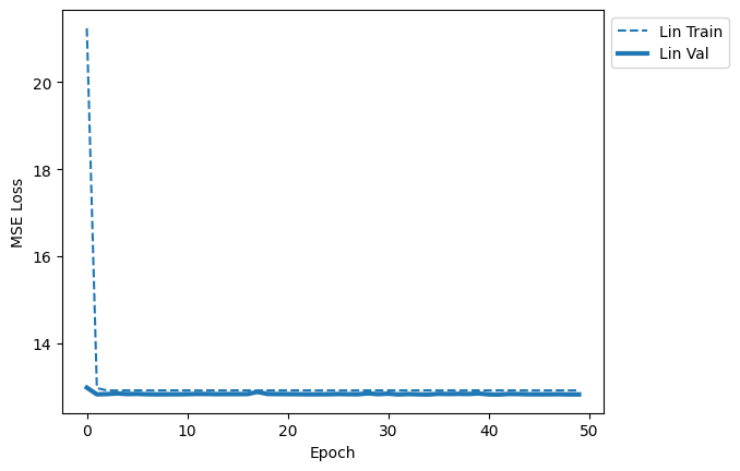
At first glance, not much learning appears to be happening.
Next let’s try the CNN.
seq_len = len(train_df['seq'].values[0])

# create Linear model object
model_cnn = DNA_CNN(seq_len)
model_cnn.to(DEVICE) # put on GPU

# run the model with default settings!
cnn_train_losses, cnn_val_losses = run_training(
    train_dl,
    val_dl,
    model_cnn,
    DEVICE
)
E0 | train loss: 14.640 | val loss: 10.167
E1 | train loss: 8.625 | val loss: 7.035
E2 | train loss: 6.305 | val loss: 4.967
E3 | train loss: 4.507 | val loss: 3.257
E4 | train loss: 3.123 | val loss: 2.256
E5 | train loss: 2.408 | val loss: 2.627
E6 | train loss: 1.997 | val loss: 2.078
E7 | train loss: 1.827 | val loss: 4.446
E8 | train loss: 1.547 | val loss: 1.297
E9 | train loss: 1.438 | val loss: 1.185
E10 | train loss: 1.249 | val loss: 1.108
E11 | train loss: 1.200 | val loss: 1.149
E12 | train loss: 1.140 | val loss: 1.096
E13 | train loss: 1.011 | val loss: 1.102
E14 | train loss: 1.022 | val loss: 1.188
E15 | train loss: 1.027 | val loss: 1.119
E16 | train loss: 1.045 | val loss: 1.040
E17 | train loss: 0.999 | val loss: 1.052
E18 | train loss: 0.965 | val loss: 1.069
E19 | train loss: 0.944 | val loss: 1.208
E20 | train loss: 0.945 | val loss: 1.175
E21 | train loss: 0.925 | val loss: 1.038
E22 | train loss: 0.927 | val loss: 1.249
E23 | train loss: 0.938 | val loss: 1.022
E24 | train loss: 0.917 | val loss: 1.042
E25 | train loss: 0.930 | val loss: 1.062
E26 | train loss: 0.917 | val loss: 1.089
E27 | train loss: 0.913 | val loss: 1.286
E28 | train loss: 0.932 | val loss: 1.041
E29 | train loss: 0.890 | val loss: 1.126
E30 | train loss: 0.903 | val loss: 1.038
E31 | train loss: 0.918 | val loss: 1.033
E32 | train loss: 0.914 | val loss: 1.048
E33 | train loss: 0.913 | val loss: 1.060
E34 | train loss: 0.900 | val loss: 1.236
E35 | train loss: 0.890 | val loss: 1.030
E36 | train loss: 0.901 | val loss: 1.066
E37 | train loss: 0.895 | val loss: 1.055
E38 | train loss: 0.914 | val loss: 1.030
E39 | train loss: 0.894 | val loss: 1.024
E40 | train loss: 0.903 | val loss: 1.056
E41 | train loss: 0.897 | val loss: 1.089
E42 | train loss: 0.917 | val loss: 1.031
E43 | train loss: 0.904 | val loss: 1.105
E44 | train loss: 0.894 | val loss: 1.284
E45 | train loss: 0.903 | val loss: 1.648
E46 | train loss: 0.904 | val loss: 1.042
E47 | train loss: 0.909 | val loss: 1.052
E48 | train loss: 0.891 | val loss: 1.186
E49 | train loss: 0.891 | val loss: 1.075cnn_data_label = (cnn_train_losses,cnn_val_losses,"CNN")
quick_loss_plot([lin_data_label,cnn_data_label])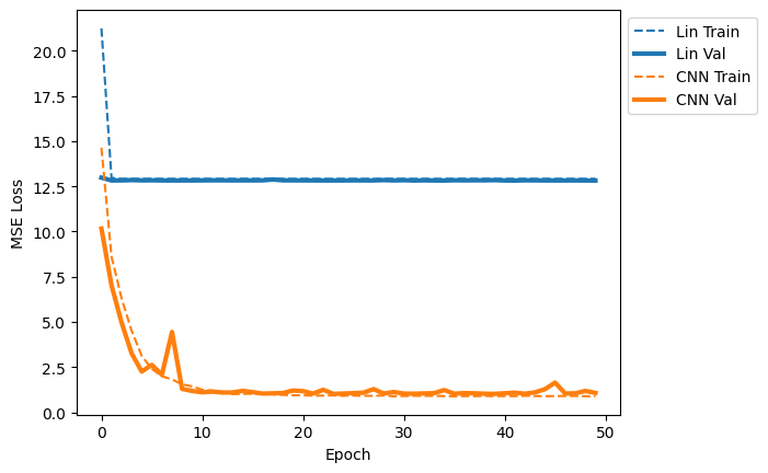
It seems clear from the loss curves that the CNN is able to capture a pattern in the data that the Linear model is not! Let’s spot check a few sequences to see what’s going on.
# oracle dict of true score for each seq
oracle = dict(mer8[['seq','score']].values)

def quick_seq_pred(model, desc, seqs, oracle):
    '''
    Given a model and some sequences, get the model's predictions
    for those sequences and compare to the oracle (true) output
    '''
    print(f"__{desc}__")
    for dna in seqs:
        s = torch.tensor(one_hot_encode(dna)).unsqueeze(0).to(DEVICE)
        pred = model(s.float())
        actual = oracle[dna]
        diff = pred.item() - actual
        print(f"{dna}: pred:{pred.item():.3f} actual:{actual:.3f} ({diff:.3f})")

def quick_8mer_pred(model, oracle):
    seqs1 = ("poly-X seqs",['AAAAAAAA', 'CCCCCCCC','GGGGGGGG','TTTTTTTT'])
    seqs2 = ("other seqs", ['AACCAACA','CCGGTGAG','GGGTAAGG', 'TTTCGTTT'])
    seqsTAT = ("with TAT motif", ['TATAAAAA','CCTATCCC','GTATGGGG','TTTATTTT'])
    seqsGCG = ("with GCG motif", ['AAGCGAAA','CGCGCCCC','GGGCGGGG','TTGCGTTT'])
    TATGCG =  ("both TAT and GCG",['ATATGCGA','TGCGTATT'])

    for desc,seqs in [seqs1, seqs2, seqsTAT, seqsGCG, TATGCG]:
        quick_seq_pred(model, desc, seqs, oracle)
        print()
# Ask the trained Linear model to make
# predictions for some 8-mers
quick_8mer_pred(model_lin, oracle)__poly-X seqs__
AAAAAAAA: pred:23.415 actual:20.000 (3.415)
CCCCCCCC: pred:13.762 actual:17.000 (-3.238)
GGGGGGGG: pred:7.189 actual:14.000 (-6.811)
TTTTTTTT: pred:17.841 actual:11.000 (6.841)
__other seqs__
AACCAACA: pred:18.987 actual:18.875 (0.112)
CCGGTGAG: pred:12.330 actual:15.125 (-2.795)
GGGTAAGG: pred:14.006 actual:15.125 (-1.119)
TTTCGTTT: pred:14.945 actual:12.125 (2.820)
__with TAT motif__
TATAAAAA: pred:22.317 actual:27.750 (-5.433)
CCTATCCC: pred:17.059 actual:25.875 (-8.816)
GTATGGGG: pred:12.329 actual:24.000 (-11.671)
TTTATTTT: pred:18.331 actual:22.125 (-3.794)
__with GCG motif__
AAGCGAAA: pred:16.972 actual:8.125 (8.847)
CGCGCCCC: pred:12.467 actual:6.250 (6.217)
GGGCGGGG: pred:8.121 actual:4.375 (3.746)
TTGCGTTT: pred:13.014 actual:2.500 (10.514)
__both TAT and GCG__
ATATGCGA: pred:15.874 actual:15.875 (-0.001)
TGCGTATT: pred:14.779 actual:13.625 (1.154)
From the above examples, it appears that the Linear model is really underpredicting sequences with a lot of G’s and overpredicting those with many T’s. This is probably because it noticed GCG made sequences have unusually low scores and TAT made sequences have unusually high scores, however since the Linear model doesn’t have a way to take into account the different context of GCG vs GAG, it just predicts that sequences with G’s should be lower. We know from our scoring scheme that this isn’t the case: it’s not that G’s in general are detrimental, but specifically GCG is.
# Ask the trained CNN model to make
# predictions for some 8-mers
quick_8mer_pred(model_cnn, oracle)
__poly-X seqs__
AAAAAAAA: pred:19.649 actual:20.000 (-0.351)
CCCCCCCC: pred:16.750 actual:17.000 (-0.250)
GGGGGGGG: pred:13.576 actual:14.000 (-0.424)
TTTTTTTT: pred:10.895 actual:11.000 (-0.105)
__other seqs__
AACCAACA: pred:18.645 actual:18.875 (-0.230)
CCGGTGAG: pred:14.759 actual:15.125 (-0.366)
GGGTAAGG: pred:15.118 actual:15.125 (-0.007)
TTTCGTTT: pred:11.789 actual:12.125 (-0.336)
__with TAT motif__
TATAAAAA: pred:26.103 actual:27.750 (-1.647)
CCTATCCC: pred:24.256 actual:25.875 (-1.619)
GTATGGGG: pred:22.838 actual:24.000 (-1.162)
TTTATTTT: pred:20.555 actual:22.125 (-1.570)
__with GCG motif__
AAGCGAAA: pred:9.007 actual:8.125 (0.882)
CGCGCCCC: pred:7.091 actual:6.250 (0.841)
GGGCGGGG: pred:5.275 actual:4.375 (0.900)
TTGCGTTT: pred:3.411 actual:2.500 (0.911)
__both TAT and GCG__
ATATGCGA: pred:15.389 actual:15.875 (-0.486)
TGCGTATT: pred:13.185 actual:13.625 (-0.440)
The CNN however is better able to adapt to the differences between 3-mer motifs! It predicts quite well on both the sequences with and without motifs.
Question 2
Compare the performance of the Linear and CNN models by using different learning rates. First run both models with higher learning rates (0.05, 0.1) and lower learning rates (0.005, 0.001), then create loss plots showing: - Linear model with these learning rates - CNN model with these learning rates
Then analyze your results by answering: 1. How does changing the learning rate affect convergence for each model? 2. Which model is more sensitive to learning rate changes, and why? 3. Based on your analysis, what learning rate would you recommend for each model type, and why?
## 6. Check model predictions on the test set An important evaluation step in machine learning tasks is to check if your model can make good predictions on the test set, which it never saw during training. Here, we can use a parity plot to visualize the difference between the actual sequence scores vs the model’s predicted scores.
#%pip install altair ## datapaneimport altair as alt
from sklearn.metrics import r2_score
## import datapane as dp ## compatibility issues with pandas version
import os
def parity_plot(model_name,df,r2):
    '''
    Given a dataframe of samples with their true and predicted values,
    make a scatterplot.
    '''
    plt.scatter(df['truth'].values, df['pred'].values, alpha=0.2)

    # y=x line
    xpoints = ypoints = plt.xlim()
    plt.plot(xpoints, ypoints, linestyle='--', color='k', lw=2, scalex=False, scaley=False)

    plt.ylim(xpoints)
    plt.ylabel("Predicted Score",fontsize=14)
    plt.xlabel("Actual Score",fontsize=14)
    plt.title(f"{model_name} (r2:{r2:.3f})",fontsize=20)
    plt.show()


def alt_parity_plot(model, df, r2, datapane=False):
    '''
    Make an interactive parity plot with altair
    '''
    import os
    import altair as alt

    os.makedirs('alt_out', exist_ok=True)

    # Convert model name to string to avoid any issues
    model = str(model)

    # Create a clean version of the dataframe
    plot_df = pd.DataFrame({
        'truth': df['truth'].astype(float),
        'pred': df['pred'].astype(float),
        'seq': df['seq'].astype(str)
    })

    # Create chart
    chart = alt.Chart(plot_df).mark_point().encode(
        x=alt.X('truth', type='quantitative', title='True Values'),
        y=alt.Y('pred', type='quantitative', title='Predictions'),
        tooltip=['seq']
    ).properties(
        title=str(f'{model} (r2:{r2:.3f})')
    )

    chart.save(f'alt_out/parity_plot_{model}.html')
    display(chart)


def parity_pred(models, seqs, oracle,alt=False,datapane=False):
    '''Given some sequences, get the model's predictions '''
    dfs = {} # key: model name, value: parity_df


    for model_name,model in models:
        print(f"Running {model_name}")
        data = []
        for dna in seqs:
            s = torch.tensor(one_hot_encode(dna)).unsqueeze(0).to(DEVICE)
            actual = oracle[dna]
            pred = model(s.float())
            data.append([dna,actual,pred.item()])
        df = pd.DataFrame(data, columns=['seq','truth','pred'])
        r2 = r2_score(df['truth'],df['pred'])
        dfs[model_name] = (r2,df)

        #plot parity plot
        if alt: # make an altair plot
            alt_parity_plot(model_name, df, r2,datapane=datapane)

        else:
            parity_plot(model_name, df, r2)
seqs = test_df['seq'].values
models = [
("Linear", model_lin),
("CNN", model_cnn)
]
parity_pred(models, seqs, oracle)Running Linear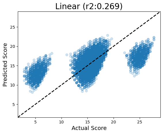
Running CNN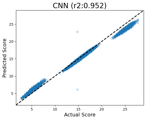
Parity plots are useful for visualizing how well your model predicts individual sequences: in a perfect model, they would all land on the y=x line, meaning that the model prediction was exactly the sequence’s actual value. But if it is off the y=x line, it means the model is over- or under-predicting.
In the Linear model, we can see that it can somewhat predict a trend in the Test set sequences, but really gets confused by these buckets of sequences in the high and low areas of the distribution (the ones with a motif).
However for the CNN, it is much better at predicting scores close to the actual value! This is expected, given that the architecture of our CNN uses 3-mer kernels to scan along the sequence for influential motifs.
But the CNN isn’t perfect. We could probably train it longer or adjust the hyperparameters, but the goal here isn’t perfection - this is a very simple task relative to actual regulatory grammars. Instead, I thought it would be interesting to use the Altair visualization library to interactively inspect which sequences the models get wrong:
alt.data_transformers.disable_max_rows() # disable altair warning
parity_pred(models, seqs, oracle,alt=True)
Running LinearRunning CNNIf you’re viewing this notebook in interactive mode and run the above cell (just viewing via the github preview will omit the altair plot in the rendering), you can hover over the points and see the individual 8-mer sequences (you can also pan and zoom in this plot).
Notice that the sequences that are off the diagonal tend to have multiple instance of the motifs! In the scoring function, we only gave the sequence a +/- bump if it had at least 1 motif, but it certainly would have been reasonable to decide to add multiple bonuses if the motif was present multiple times. In this example, I arbitrarily only added the bonus for at least 1 motif occurrence, but we could have made a different scoring function.
In any case, I thought it was cool that the model noticed the multiple occurrences and predicted them to be important. I suppose we did fool it a little, though an R2 of 0.95 is pretty respectable :)
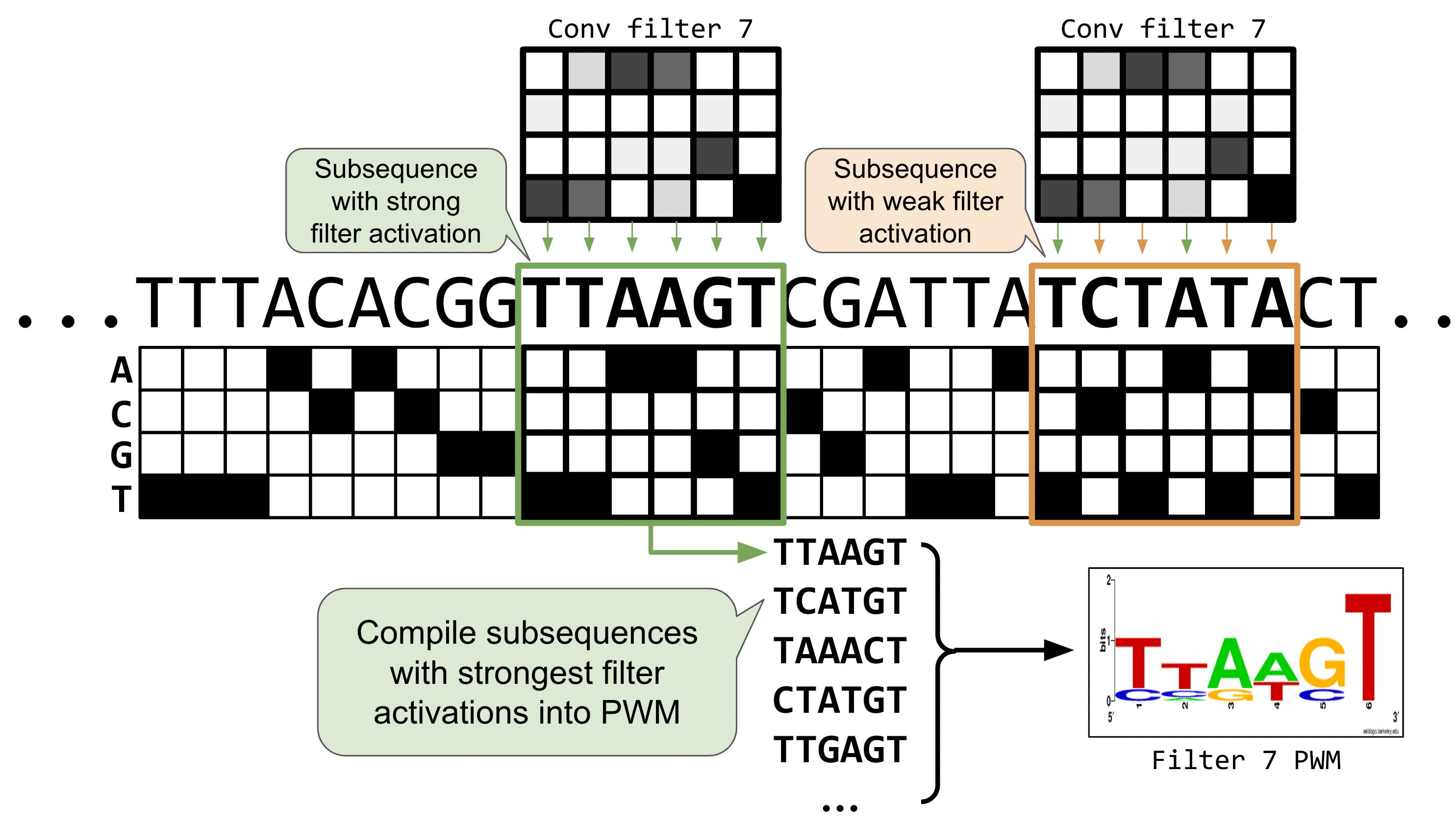
## 7. Visualize convolutional filters When training CNN models, it can be useful to visualize the first layer convolutional filters to try to understand more about what the model is learning. With image data, the first layer convolutional filters often learn patterns such as borders or colors or textures - basic image elements that can be recombined to make more complex features.
In DNA, convolutional filters can be thought of like motif scanners. Similar to a position weight matrix for visualizing sequence logos, a convolutional filter is like a matrix showing a particular DNA pattern, but instead of being an exact sequence, it can hold some uncertainty about which nucleotides show up in which part of the pattern. Some positions might be very certain (i.e., there’s always an A in position 2; high information content) while other positions could hold a variety of nucleotides with about equal probability (high entropy; low information content).
The calculations that occur within the hidden layers of neural networks can get very complex and not every convolutional filter will be an obviously relevant pattern, but sometimes patterns in the filters do emerge and can be informative for helping to explain the model’s predictions.
Below are some functions to visualize the first layer convolutional filters, both as a raw heatmap and as a motif logo.
===
Visualizing Convolutional Filters When training convolutional neural networks (CNNs), it’s often helpful to visualize the filters in the first convolutional layer to better understand what features the model is learning from the input data.
In image data:
The first-layer filters commonly learn simple, low-level features like:
Edges or borders Color gradients Textures or basic shapes
These simple elements can be combined in deeper layers to form more complex patterns, such as object parts or entire shapes.
🧬 In DNA sequence data:
Convolutional filters act similarly to motif detectors. They can learn biologically meaningful patterns in the sequence, much like:
- Position Weight Matrices (PWMs)
- Sequence logos
Each filter can be thought of as a matrix scanning for a specific DNA pattern — not necessarily a fixed sequence, but one that may allow for some variation in certain positions.
For example:
One position in the filter might strongly prefer an “A” (indicating low entropy and high information content). Another position might tolerate any nucleotide (high entropy, low information content). These learned filters can sometimes correspond to known biological motifs, or reveal novel sequence patterns that are predictive for the task at hand (e.g., enhancer activity, binding sites, expression levels).
Question 3
Design an approach to improve the model’s prediction accuracy, particularly focusing on the sequences where the current model performs poorly:
After identifying sequences where the CNN model has high prediction errors, propose and implement a modification to either the model architecture, the loss function, the training process, or the data representation
Retrain the model with your modifications
Create comparative visualizations (such as parity plots, error histograms, or other appropriate plots) to demonstrate the impact of your changes
Analyze your results by discussing how your modification addresses the specific weaknesses you identified. What are the trade-offs involved in your approach?
import logomakerdef get_conv_layers_from_model(model):
'''
Given a trained model, extract its convolutional layers
'''
model_children = list(model.children())
# counter to keep count of the conv layers
model_weights = [] # we will save the conv layer weights in this list
conv_layers = [] # we will save the actual conv layers in this list
bias_weights = []
counter = 0
# append all the conv layers and their respective weights to the list
for i in range(len(model_children)):
# get model type of Conv1d
if type(model_children[i]) == nn.Conv1d:
counter += 1
model_weights.append(model_children[i].weight)
conv_layers.append(model_children[i])
bias_weights.append(model_children[i].bias)
# also check sequential objects' children for conv1d
elif type(model_children[i]) == nn.Sequential:
for child in model_children[i]:
if type(child) == nn.Conv1d:
counter += 1
model_weights.append(child.weight)
conv_layers.append(child)
bias_weights.append(child.bias)
print(f"Total convolutional layers: {counter}")
return conv_layers, model_weights, bias_weights
def view_filters(model_weights, num_cols=8):
model_weights = model_weights[0]
num_filt = model_weights.shape[0]
filt_width = model_weights[0].shape[1]
num_rows = int(np.ceil(num_filt/num_cols))
# visualize the first conv layer filters
plt.figure(figsize=(20, 17))
for i, filter in enumerate(model_weights):
ax = plt.subplot(num_rows, num_cols, i+1)
ax.imshow(filter.cpu().detach(), cmap='gray')
ax.set_yticks(np.arange(4))
ax.set_yticklabels(['A', 'C', 'G','T'])
ax.set_xticks(np.arange(filt_width))
ax.set_title(f"Filter {i}")
plt.tight_layout()
plt.show()First, we can take a peek at the raw filters.
conv_layers, model_weights, bias_weights = get_conv_layers_from_model(model_cnn)
view_filters(model_weights)
Total convolutional layers: 1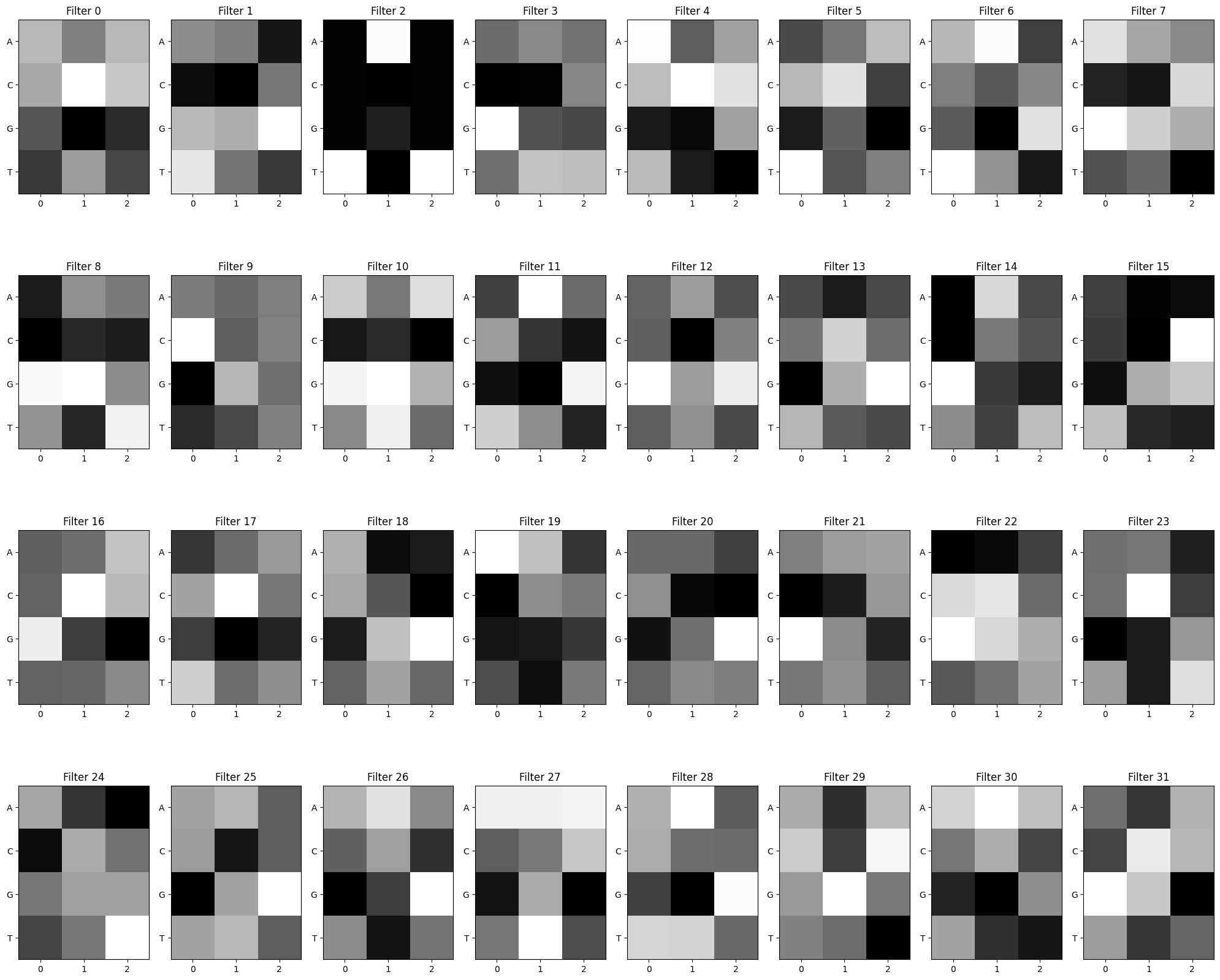
def get_conv_output_for_seq(seq, conv_layer):
    '''
    Given an input sequeunce and a convolutional layer,
    get the output tensor containing the conv filter
    activations along each position in the sequence
    '''
    # format seq for input to conv layer (OHE, reshape)
    seq = torch.tensor(one_hot_encode(seq)).unsqueeze(0).permute(0,2,1).to(DEVICE)

    # run seq through conv layer
    with torch.no_grad(): # don't want as part of gradient graph
        # apply learned filters to input seq
        res = conv_layer(seq.float())
        return res[0]


def get_filter_activations(seqs, conv_layer,act_thresh=0):
    '''
    Given a set of input sequences and a trained convolutional layer,
    determine the subsequences for which each filter in the conv layer
    activate most strongly.

    1.) Run seq inputs through conv layer.
    2.) Loop through filter activations of the resulting tensor, saving the
            position where filter activations were > act_thresh.
    3.) Compile a count matrix for each filter by accumulating subsequences which
            activate the filter above the threshold act_thresh
    '''
    # initialize dict of pwms for each filter in the conv layer
    # pwm shape: 4 nucleotides X filter width, initialize to 0.0s
    num_filters = conv_layer.out_channels
    filt_width = conv_layer.kernel_size[0]
    filter_pwms = dict((i,torch.zeros(4,filt_width)) for i in range(num_filters))

    print("Num filters", num_filters)
    print("filt_width", filt_width)

    # loop through a set of sequences and collect subseqs where each filter activated
    for seq in seqs:
        # get a tensor of each conv filter activation along the input seq
        res = get_conv_output_for_seq(seq, conv_layer)

        # for each filter and it's activation vector
        for filt_id,act_vec in enumerate(res):
            # collect the indices where the activation level
            # was above the threshold
            act_idxs = torch.where(act_vec>act_thresh)[0]
            activated_positions = [x.item() for x in act_idxs]

            # use activated indicies to extract the actual DNA
            # subsequences that caused filter to activate
            for pos in activated_positions:
                subseq = seq[pos:pos+filt_width]
                #print("subseq",pos, subseq)
                # transpose OHE to match PWM orientation
                subseq_tensor = torch.tensor(one_hot_encode(subseq)).T

                # add this subseq to the pwm count for this filter
                filter_pwms[filt_id] += subseq_tensor

    return filter_pwms

def view_filters_and_logos(model_weights,filter_activations, num_cols=8):
    '''
    Given some convolutional model weights and filter activation PWMs,
    visualize the heatmap and motif logo pairs in a simple grid
    '''
    model_weights = model_weights[0].squeeze(1)
    print(model_weights.shape)

    # make sure the model weights agree with the number of filters
    assert(model_weights.shape[0] == len(filter_activations))

    num_filts = len(filter_activations)
    num_rows = int(np.ceil(num_filts/num_cols))*2+1
    # ^ not sure why +1 is needed... complained otherwise

    plt.figure(figsize=(20, 17))

    j=0 # use to make sure a filter and it's logo end up vertically paired
    for i, filter in enumerate(model_weights):
        if (i)%num_cols == 0:
            j += num_cols

        # display raw filter
        ax1 = plt.subplot(num_rows, num_cols, i+j+1)
        ax1.imshow(filter.cpu().detach(), cmap='gray')
        ax1.set_yticks(np.arange(4))
        ax1.set_yticklabels(['A', 'C', 'G','T'])
        ax1.set_xticks(np.arange(model_weights.shape[2]))
        ax1.set_title(f"Filter {i}")

        # display sequence logo
        ax2 = plt.subplot(num_rows, num_cols, i+j+1+num_cols)
        filt_df = pd.DataFrame(filter_activations[i].T.numpy(),columns=['A','C','G','T'])
        filt_df_info = logomaker.transform_matrix(filt_df,from_type='counts',to_type='information')
        logo = logomaker.Logo(filt_df_info,ax=ax2)
        ax2.set_ylim(0,2)
        ax2.set_title(f"Filter {i}")

    plt.tight_layout()
# just use some seqs from test_df to activate filters
some_seqs = random.choices(seqs, k=3000)
filter_activations = get_filter_activations(some_seqs, conv_layers[0])
view_filters_and_logos(model_weights,filter_activations)Num filters 32
filt_width 3
torch.Size([32, 4, 3])/Users/haekyungim/miniconda3/envs/gene46100/lib/python3.12/site-packages/logomaker/src/Logo.py:1001: UserWarning: Attempting to set identical low and high ylims makes transformation singular; automatically expanding.
self.ax.set_ylim([ymin, ymax])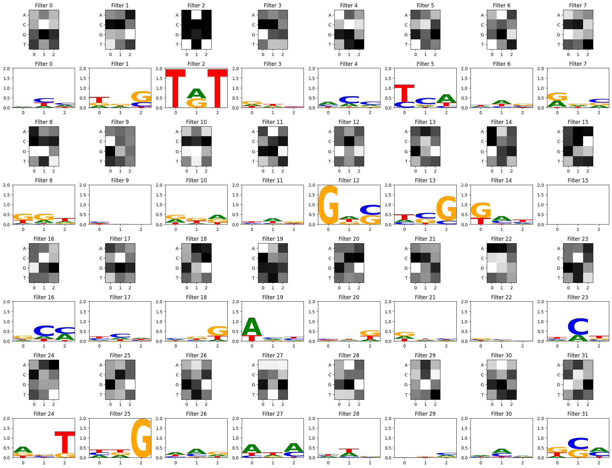
Visualize filters using a stronger activation threshold
act_thresh = 1 instead of 0. (Some filters have no subsequence matches above the threshold and result in an empty motif logo)
filter_activations = get_filter_activations(some_seqs, conv_layers[0],act_thresh=1)
view_filters_and_logos(model_weights,filter_activations)Num filters 32
filt_width 3
torch.Size([32, 4, 3])/Users/haekyungim/miniconda3/envs/gene46100/lib/python3.12/site-packages/logomaker/src/Logo.py:1001: UserWarning: Attempting to set identical low and high ylims makes transformation singular; automatically expanding.
self.ax.set_ylim([ymin, ymax])
/Users/haekyungim/miniconda3/envs/gene46100/lib/python3.12/site-packages/logomaker/src/Logo.py:1001: UserWarning: Attempting to set identical low and high ylims makes transformation singular; automatically expanding.
  self.ax.set_ylim([ymin, ymax])
/Users/haekyungim/miniconda3/envs/gene46100/lib/python3.12/site-packages/logomaker/src/Logo.py:1001: UserWarning: Attempting to set identical low and high ylims makes transformation singular; automatically expanding.
self.ax.set_ylim([ymin, ymax])
/Users/haekyungim/miniconda3/envs/gene46100/lib/python3.12/site-packages/logomaker/src/Logo.py:1001: UserWarning: Attempting to set identical low and high ylims makes transformation singular; automatically expanding.
self.ax.set_ylim([ymin, ymax])
/Users/haekyungim/miniconda3/envs/gene46100/lib/python3.12/site-packages/logomaker/src/Logo.py:1001: UserWarning: Attempting to set identical low and high ylims makes transformation singular; automatically expanding.
self.ax.set_ylim([ymin, ymax])
/Users/haekyungim/miniconda3/envs/gene46100/lib/python3.12/site-packages/logomaker/src/Logo.py:1001: UserWarning: Attempting to set identical low and high ylims makes transformation singular; automatically expanding.
self.ax.set_ylim([ymin, ymax])
/Users/haekyungim/miniconda3/envs/gene46100/lib/python3.12/site-packages/logomaker/src/Logo.py:1001: UserWarning: Attempting to set identical low and high ylims makes transformation singular; automatically expanding.
self.ax.set_ylim([ymin, ymax])
/Users/haekyungim/miniconda3/envs/gene46100/lib/python3.12/site-packages/logomaker/src/Logo.py:1001: UserWarning: Attempting to set identical low and high ylims makes transformation singular; automatically expanding.
self.ax.set_ylim([ymin, ymax])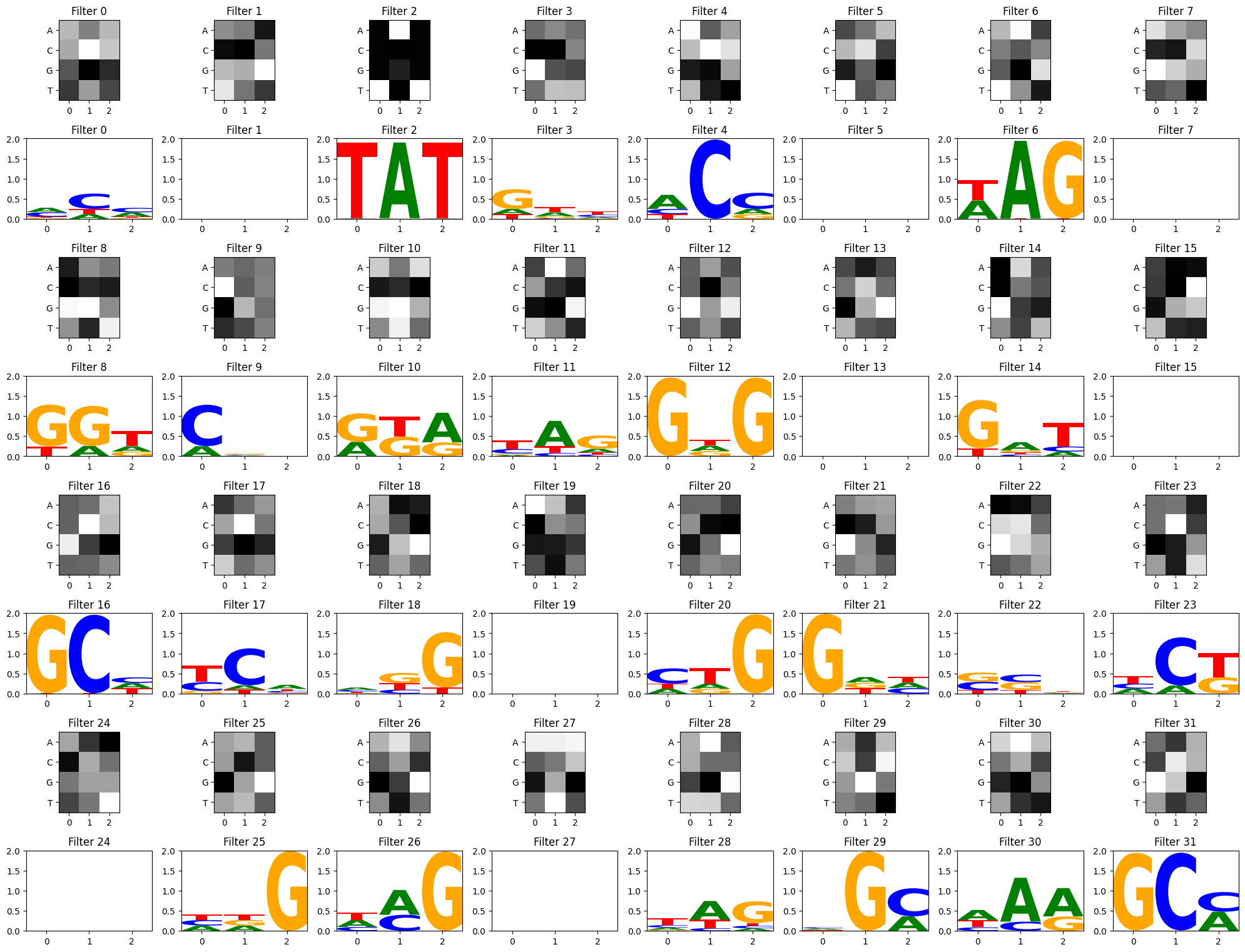
From this particular CNN training, we can see a few filters have picked up on the strong TAT and GCG motifs, but other filters have focused on other patterns as well. There is some debate about how relevant convolutional filter visualizations are for model interpretability. In deep models with multiple convolutional layers, convolutional filters can be recombined in more complex ways inside the hidden layers, so the first layer filters may not be as informative on their own (Koo and Eddy, 2019). Much of the field has since moved towards attention mechanisms and other explainability methods, but should you be curious to visualize your filters as potential motifs, these functions may help get you started!
## 8. Conclusion This tutorial shows some basic Pytorch structure for building CNN models that work with DNA sequences. The practice task used in this demo is not reflective of real biological signals; rather, we designed the scoring method to simulate the presence of regulatory motifs in very short sequences that were easy for us humans to inspect and verify that Pytorch was behaving as expected. From this small example, we observed how a basic CNN with sliding filters was able to predict our scoring scheme better than a basic linear model that only accounted for absolute nucleotide position (without local context).
To read more about CNN’s applied to DNA in the wild, check out the following foundational papers: * DeepBind: Alipanahi et al 2015 * DeepSea: Zhou and Troyanskaya 2015 * Basset: Kelley et al 2016
I hope other new-to-ML folks interested in tackling biological questions may find this helpful for getting started with using Pytorch to model DNA sequences :)