# %pip install seaborn matplotlib
# %pip install scikit-learn plotnine tqdm pandas
# %pip install numpy ## gets installed with scikit-learn
# %pip install tqdm
# %pip install torch
# %pip install torchvision torchmetricstest
notebook
Install packages for gene46100
import numpy as np
import matplotlib.pyplot as plt
def periodic_u(x_values):
"""
Calculates the periodic function u(x) = x, with period L=1.
This is equivalent to u(x) = x - floor(x) for an array of x values.
Args:
x_values (np.array): Input x values.
Returns:
np.array: Values of the periodic function.
"""
return x_values - np.floor(x_values)
def fourier_series_approx(x_values, n_terms_approx):
"""
Calculates the Fourier series approximation of u(x).
The formula derived is: u_approx(x) = 1/2 - (1/pi) * sum_{n=1}^{N} (sin(2*pi*n*x) / n)
Args:
x_values (np.array): Input x values.
n_terms_approx (int): Number of terms (N) to include in the summation.
Returns:
np.array: Values of the Fourier series approximation.
"""
# Initialize an array of zeros with the same shape as x_values to store the sum
series_sum_val = np.zeros_like(x_values, dtype=float)
# Sum the series term by term
for n_val in range(1, n_terms_approx + 1):
series_sum_val += (np.sin(2 * np.pi * n_val * x_values)) / n_val
# Apply the full formula
approximation = 0.5 - (1 / np.pi) * series_sum_val
return approximation
# --- Parameters for plotting ---
N_TERMS_IN_SERIES = 100 # Number of terms in the Fourier series approximation
X_PLOT_MIN = 0 # Minimum x value for plotting
X_PLOT_MAX = 3 # Maximum x value for plotting (to show 3 periods)
NUM_POINTS_PLOT = 1000 # Number of points for generating smooth plot lines
# --- Generate x values for plotting ---
# Using linspace to create an array of evenly spaced x values
x_plot_values = np.linspace(X_PLOT_MIN, X_PLOT_MAX, NUM_POINTS_PLOT)
# --- Calculate y values for the original periodic function ---
y_original_periodic = periodic_u(x_plot_values)
# --- Calculate y values for the Fourier series approximation ---
y_fourier_approximation = fourier_series_approx(x_plot_values, N_TERMS_IN_SERIES)
# --- Plotting the results ---
plt.figure(figsize=(14, 8)) # Create a figure with a specified size for better readability
# Plot the original periodic function
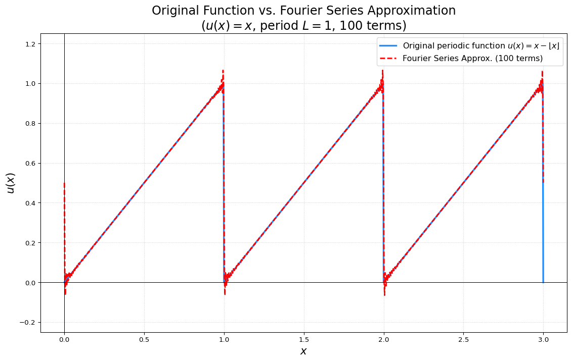
plt.plot(x_plot_values, y_original_periodic, label='Original periodic function $u(x) = x - \\lfloor x \\rfloor$', color='dodgerblue', linewidth=2.5)
# Plot the Fourier series approximation
plt.plot(x_plot_values, y_fourier_approximation, label=f'Fourier Series Approx. ({N_TERMS_IN_SERIES} terms)', color='red', linestyle='--', linewidth=2)
# --- Adding plot enhancements ---
plt.title(f'Original Function vs. Fourier Series Approximation\n($u(x)=x$, period $L=1$, {N_TERMS_IN_SERIES} terms)', fontsize=18)
plt.xlabel('$x$', fontsize=16)
plt.ylabel('$u(x)$', fontsize=16)
plt.legend(fontsize=12, loc='upper right')
plt.grid(True, linestyle=':', alpha=0.6) # Add a grid for easier value reading
plt.ylim(-0.25, 1.25) # Set y-axis limits to focus on the function's range
plt.axhline(0, color='black', linewidth=0.75) # Add a horizontal line at y=0
plt.axvline(0, color='black', linewidth=0.75) # Add a vertical line at x=0
# Add text annotations for clarity if needed, e.g., pointing out Gibbs phenomenon
# plt.annotate('Gibbs Phenomenon', xy=(1, 0.9), xytext=(1.2, 0.7),
# arrowprops=dict(facecolor='black', shrink=0.05), fontsize=10)
# Display the plot
plt.show()