Quick Introduction to Deep Learning

GENE 46100 — Unit 00

Haky Im

2025-03-25

Course Roadmap

Unit	Question	Topic	Weeks
0	What is DL? Can we detect regulatory motifs in DNA?	MLP, CNN, DNA scoring	1–3
1	Can we learn the “language” of DNA?	Transformers & Genomic GPT	4–5
2	Can we predict gene regulation from sequence?	Enformer & Borzoi	6–7
3	Can we model microbial communities?		8–9

Tools we’ll use:

• Python + PyTorch
• Google Colab (GPU)
• Weights & Biases

By the end: You’ll understand how state-of-the-art models predict gene expression from DNA sequence and apply DL to microbiome and other areas.

What Can Deep Learning Do in Genomics?

• Predict TF binding from DNA sequence alone
• Score regulatory variants without experiments
• Predict gene expression from 200kb of sequence (Enformer)
• Generate protein structures (AlphaFold)
• Build DNA language models that learn grammar of the genome

These models learn patterns we didn’t know to look for.

Today’s Learning Objectives

1. Understand and implement gradient descent to fit a linear model
2. See why linear models fail on nonlinear data
3. Build a multi-layer perceptron (MLP) that succeeds
4. Learn the basics of PyTorch: model, loss, optimizer

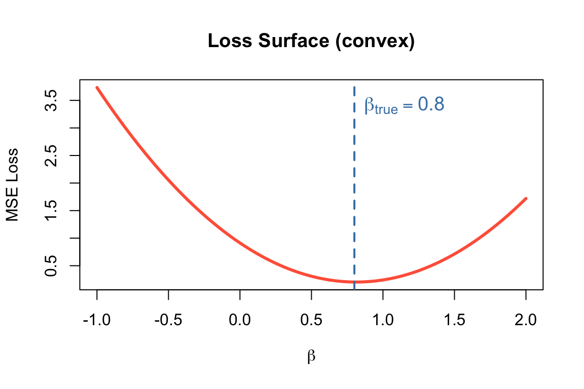
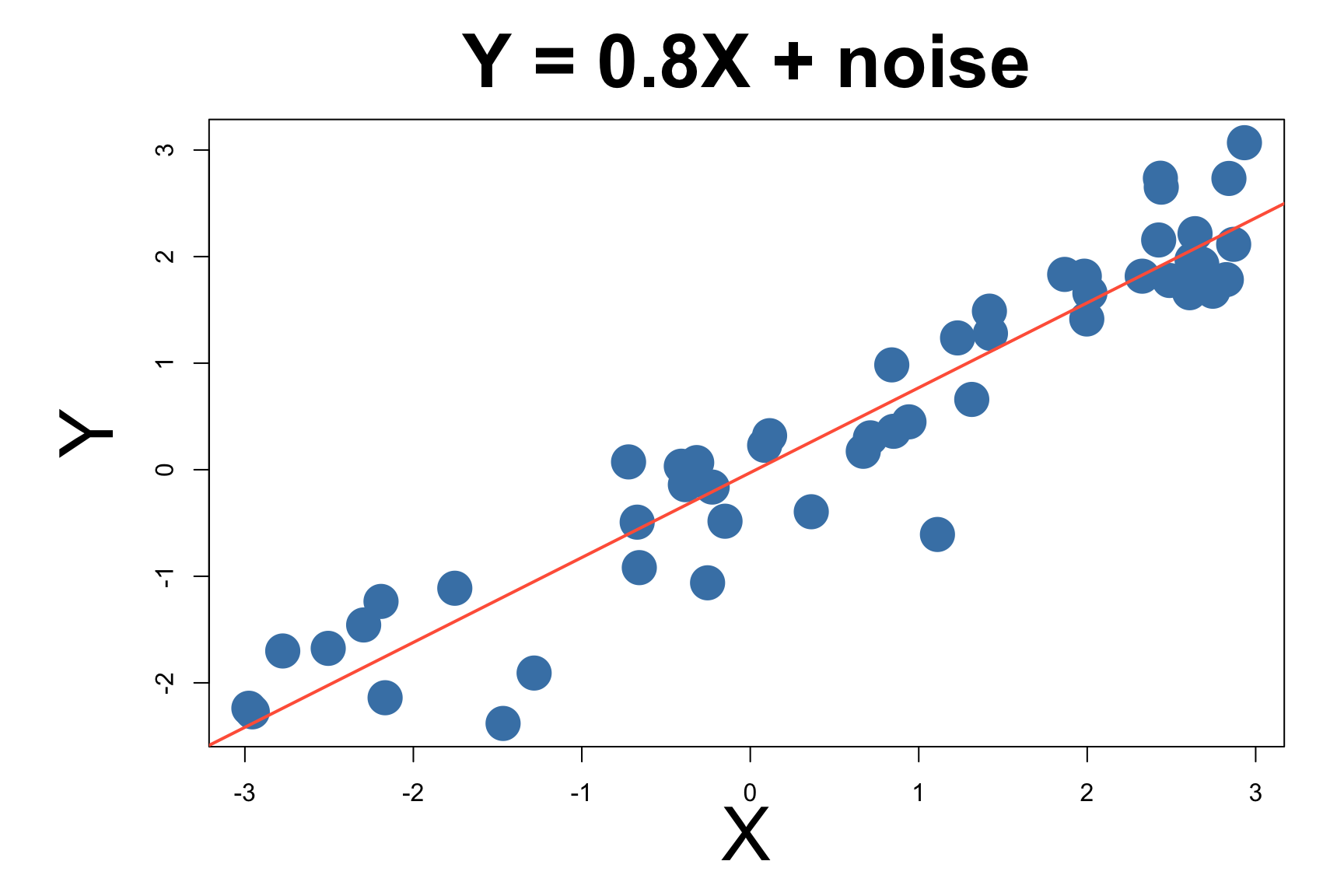
Let’s start with a linear model

\[y = X\beta + \epsilon ~~~~~ \text{where }\epsilon \sim N(0, \sigma)\]

Linear Model Has Closed Form Solution

For linear regression, there’s a closed-form solution:

\[\hat{\beta} = (X^TX)^{-1}X^Ty\] this is called the normal equation.

Estimated: \(\hat{\beta} \approx\) true \(\beta\)

Most Models Don’t Have Closed Form Solutions

The normal equation works for linear models…

• Neural networks with millions of parameters
• Nonlinear activation functions
• Complex architectures

We need a general-purpose optimization method.

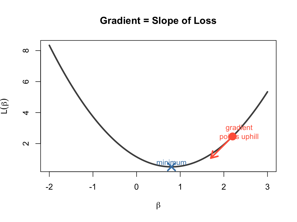
What is a Gradient?

A gradient is the derivative of a function — it tells us the slope.

\[f'(\beta) = \lim_{\Delta\beta \to 0} \frac{f(\beta + \Delta\beta) - f(\beta)}{\Delta\beta}\]

• Positive gradient → function is increasing → move left
• Negative gradient → function is decreasing → move right
• Zero gradient → you’re at a minimum (or maximum)

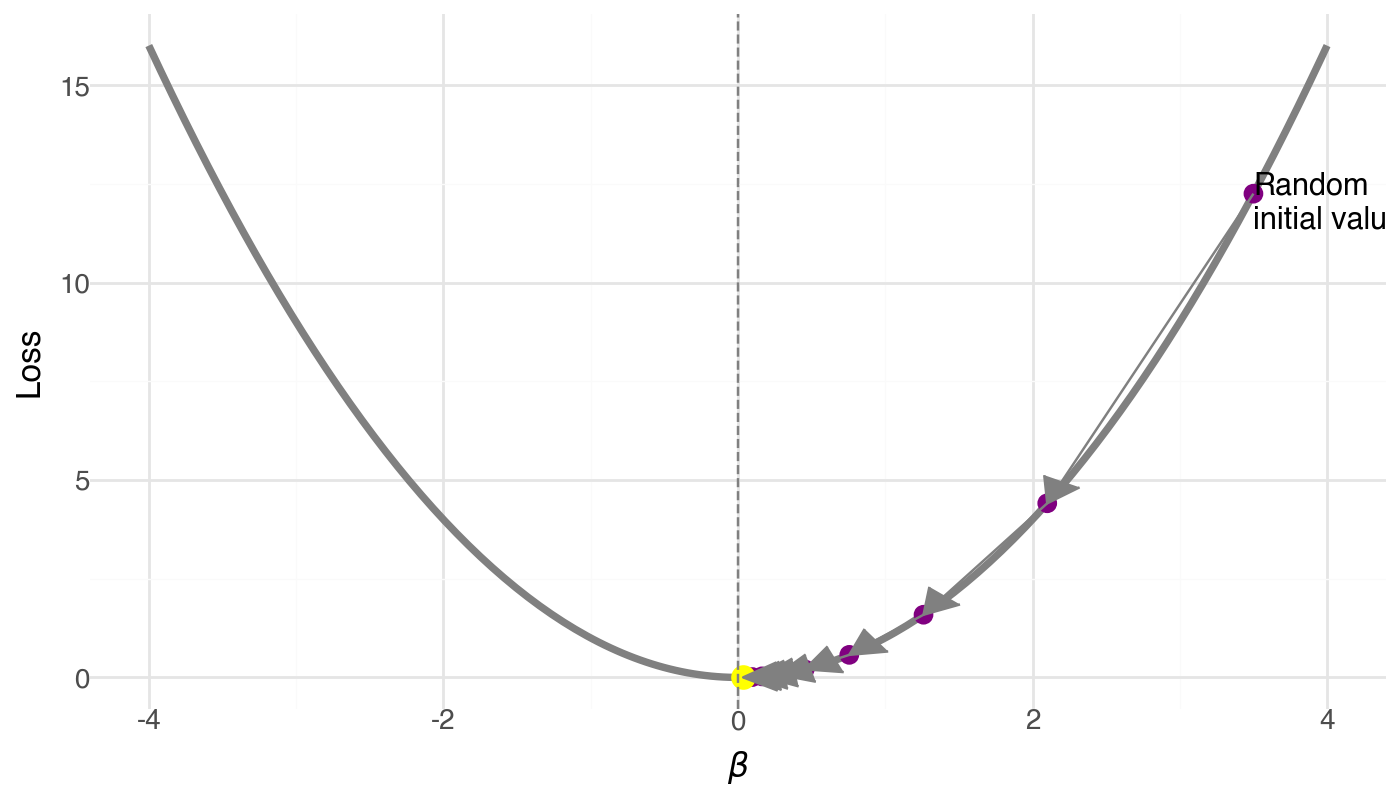
Gradient Descent: Follow the Slope Downhill

Algorithm:

1. Start at a random \(\beta\) (high loss)
2. Compute the gradient (slope)
3. Take a step opposite to the gradient
4. Repeat until convergence

\(\beta_{t+1} = \beta_t - \alpha \cdot \nabla L(\beta_t)\)

\(\alpha\) = learning rate (step size)

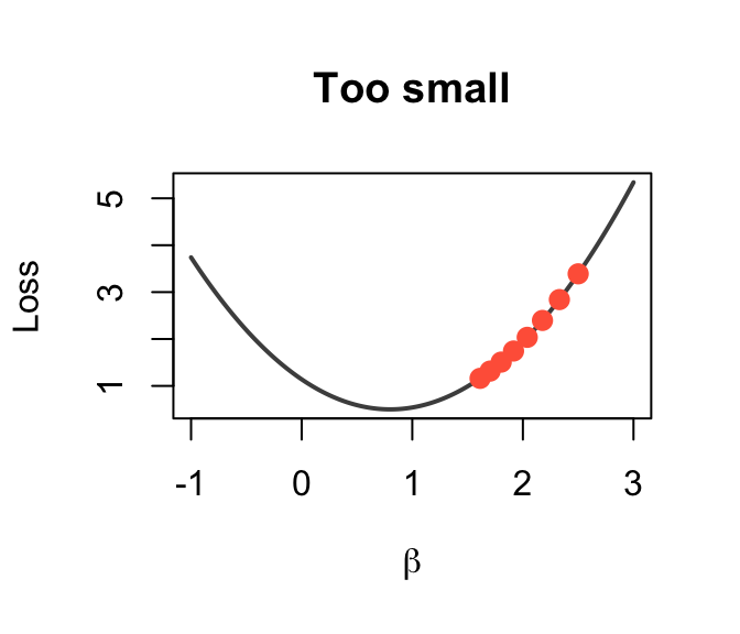
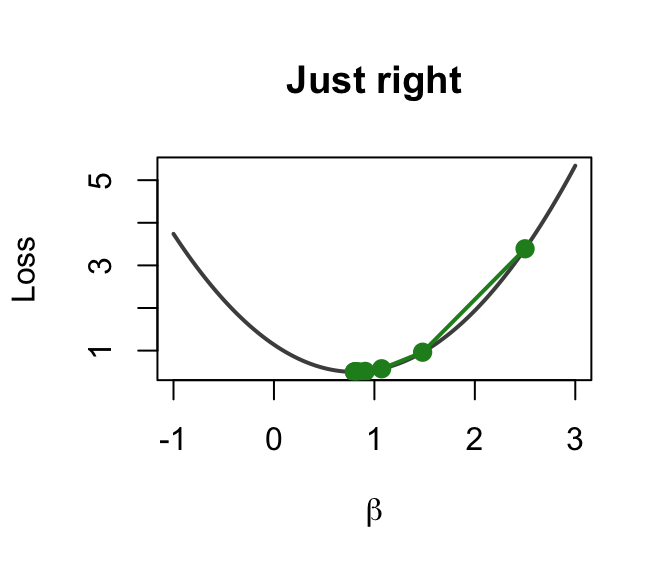
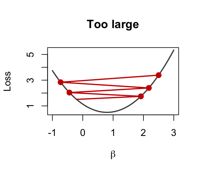
The Learning Rate \(\alpha\)

Too small (\(\alpha = 0.0001\))

Just right (\(\alpha = 0.003\))

Too large (\(\alpha = 0.1\))

Tiny steps → very slow

Smooth convergence

Overshoots → diverges!

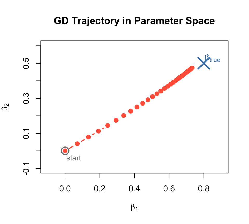
GD Trajectory: Watching \(\beta\) Converge

With 2 parameters (\(\beta_1\), \(\beta_2\)), gradient descent traces a path through parameter space:

for _ in range(50):
    diff = x.dot(b) - y
    grad = diff.dot(x) / n
    b -= lr * grad

The trajectory spirals toward the true \(\beta\).

Stochastic Gradient Descent (SGD)

In practice, computing gradients on all data is expensive.

Solution: use a random mini-batch at each step. \[\nabla L \approx \frac{1}{|B|} \sum_{i \in B} \nabla L_i\]

Stochastic Gradient Descent (SGD)

Full-batch GD:

• Exact gradient
• Slow per step
• Smooth path

SGD (mini-batch):

• Approximate gradient
• Fast per step
• Noisy but effective path

The noise actually helps escape bad local minima!

Three Components of Machine Learning

Every ML model needs these three ingredients:

• Model — \(\hat{y} = f(x)\): defines the hypothesis
• Loss — \(L(\hat{y}, y)\): measures how wrong we are
• Optimizer — \(\beta \leftarrow \beta - \alpha \nabla L\): updates params to reduce loss

Component	Linear regression	Neural network
Model	\(y = X\beta\)	\(y = W_2 \sigma(W_1 x + b_1) + b_2\)
Loss	MSE	MSE, cross-entropy, …
Optimizer	Normal equation	SGD, Adam, …

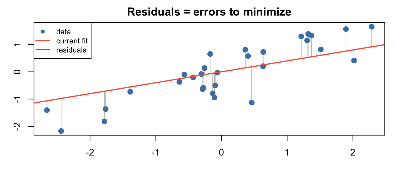
The Loss Function: MSE

Mean Squared Error: \[L(\beta) = \frac{1}{m}\sum_{i=1}^{m} (\hat{y}^{(i)} - y^{(i)})^2\]

Its gradient (for linear model):

\[\frac{\partial L}{\partial \beta_j} = \frac{1}{m}\sum_{i} (\hat{y}^{(i)} - y^{(i)}) \cdot x_j^{(i)}\]

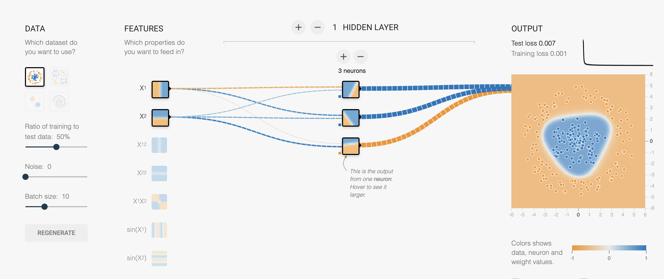
See It Live: Fit a Line in the Playground

Open playground.hakyimlab.org

Settings:

• Problem type → Regression
• Dataset → reg-plane (linear data)
• 1 hidden neuron, Linear activation
• Hit ▶ Play

Watch the loss curve drop as the gradient descent finds the optimal \(w\) and \(b\).

Try changing the learning rate — see it converge faster or explode.

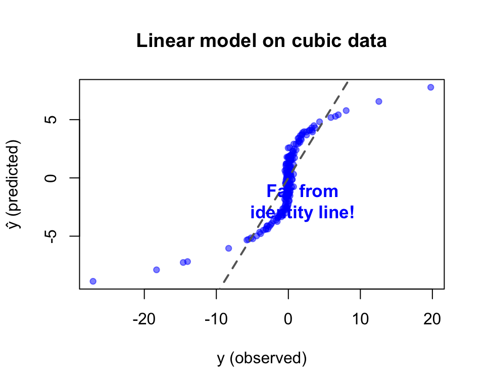
Linear Model Succeeds — On Linear Data

The playground fits \(y = wx + b\) perfectly on the linear dataset.

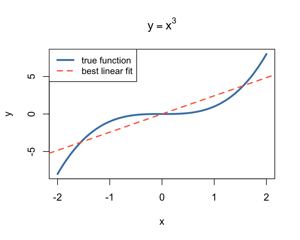
But what if the data isn’t linear?

The best possible linear fit to \(y = x^3\) is still terrible.

No amount of training will fix this — the model is wrong, not the optimizer.

Try Cubic Data in the Playground

Switch to dataset → Cubic (\(y \approx x^3\))

Keep: 1 neuron, Linear activation

Hit ▶ Play and wait…

Loss stays high. The best linear fit is a flat plane through a curve.

No matter how long you train — a linear model can’t bend.

We need a model that can learn any shape

• A model that can learn any shape
• Without us specifying the functional form
• From data alone

Solution: add nonlinearity → build a neural network.

Multi-Layer Perceptron (MLP)

A neural network with:

• Input layer: your features
• Hidden layer(s): with nonlinear activation
• Output layer: prediction

\[y = W_2 \cdot \sigma(W_1 x + b_1) + b_2\]

Key insight: \(\sigma\) (activation function) introduces the bends that let the model fit curves.

What Does a Neuron Do?

                      activation
  x₁ ──w₁──┐         function
             ├──▶ Σ ──▶ σ(·) ──▶ output
  x₂ ──w₂──┘  +b

Without activation (linear):

\(\text{output} = w_1 x_1 + w_2 x_2 + b\)

Just a weighted sum — still a line!

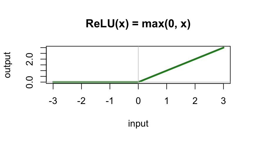
With ReLU activation:

\(\text{output} = \max(0, w_1 x_1 + w_2 x_2 + b)\)

Now it can produce a kink — a bent line!

Building Up: 2 Neurons = 2 Bends

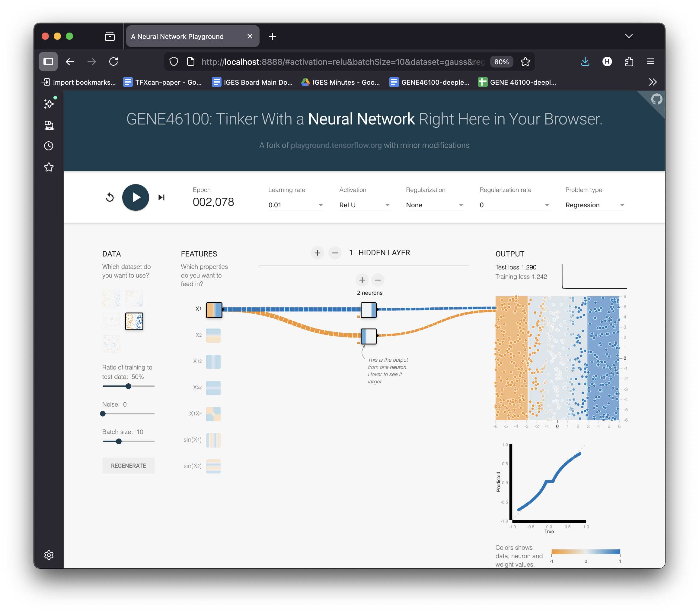
Change activation → ReLU

Set hidden layer → 2 neurons

Hit ▶ Play

Select Pred vs True to show the scatter plot

Each neuron contributes one ReLU “kink.” Combined, they approximate a curve — but it’s rough.

Loss is lower, but the fit isn’t great yet.

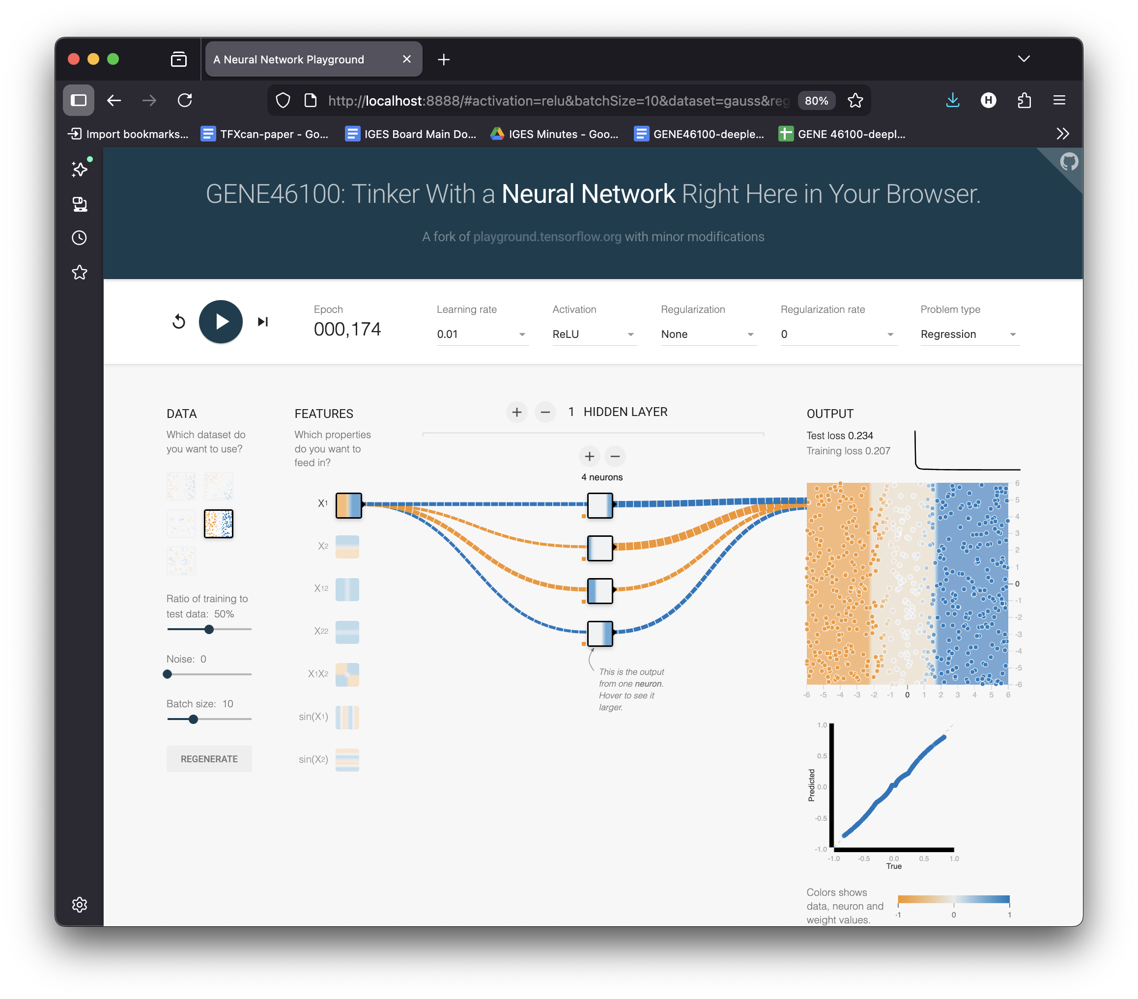
4 Neurons = 4 Bends = Smoother

Increase to 4 neurons

Hit ▶ Play

Select Pred vs True to show the scatter plot

More neurons = more “kinks” = smoother approximation of \(x^3\).

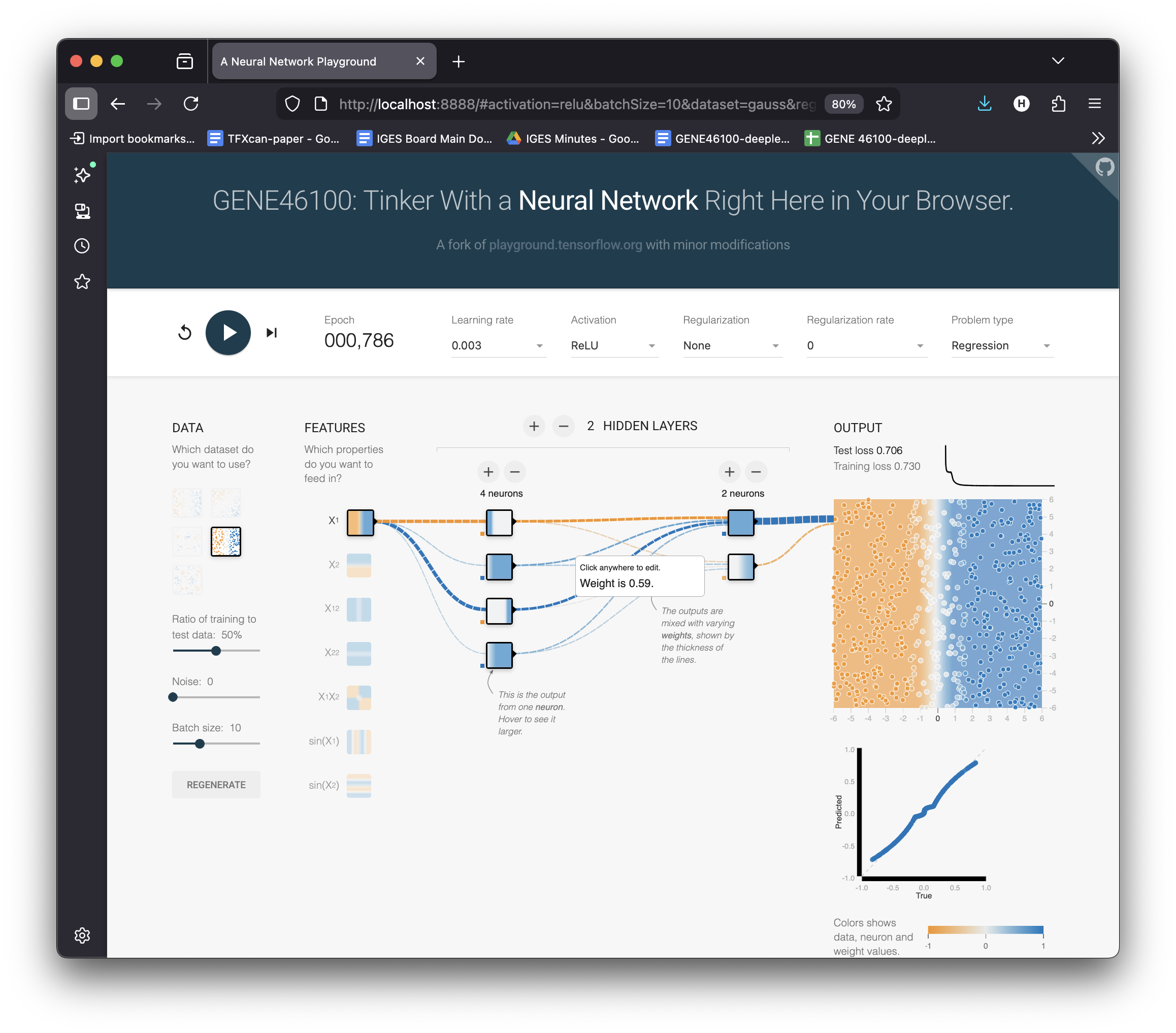
Adding Depth: 2 Layers (4 → 2)

Add a second layer: 4 neurons → 2 neurons

Hit ▶ Play

Layer 1 learns basic bends → Layer 2 combines them into a smooth curve.

Stacking layers = composing simple features into complex functions.

The MLP Progression — Summary

  LINEAR (1 neuron, no activation)          2 NEURONS + ReLU
  ┌────────────────────────┐                ┌────────────────────────┐
  │     ──────────────     │                │     ─────╱             │
  │   flat line            │                │         ╱──────        │
  │   can't bend!          │                │   two bends            │
  └────────────────────────┘                └────────────────────────┘

  4 NEURONS + ReLU                          2 LAYERS (4→2) + ReLU
  ┌────────────────────────┐                ┌────────────────────────┐
  │         ╱‾‾‾╲          │                │        ╱‾‾‾╲           │
  │   ─────╱     ╲─────    │                │  ─────╱     ╲─────     │
  │   four bends           │                │   smooth curve         │
  └────────────────────────┘                └────────────────────────┘

A neural network approximates any function by combining simple bent lines.

Counting Parameters

Exercise: count parameters for this network:

• Input: 2 features
• Hidden: 3 neurons
• Output: 1

  x₁ ──┬──▶ h₁ ──┐
       ├──▶ h₂ ──┼──▶ ŷ
  x₂ ──┴──▶ h₃ ──┘

. . .

Layer 1: 2×3 weights + 3 biases = 9

Layer 2: 3×1 weights + 1 bias = 4

Total: 13 parameters

Manually computing gradients for 13 parameters is tedious. For millions? Impossible.

This is why we need PyTorch.

Why the Activation Function Matters

Without activation, stacking layers is pointless:

\[W_2(W_1 x) = (W_2 W_1) x = W'x\]

Any number of linear layers = one linear layer!

Try it yourself: set activation to “Linear” in the playground. Add as many layers as you want — the output is always a flat gradient.

Why the Activation Function Matters

The activation function breaks linearity, allowing each layer to add new “bends.”

Common activations:

• ReLU: \(\max(0, x)\) — fast, simple
• Tanh: \(\frac{e^x - e^{-x}}{e^x + e^{-x}}\) — S-curve
• Sigmoid: \(\frac{1}{1+e^{-x}}\) — for probabilities

Universal Approximation Theorem

An MLP with a single hidden layer can approximate any continuous function to arbitrary accuracy, given enough hidden neurons.

In playground terms: with enough neurons, you have enough bends to trace any curve.

What this doesn’t tell you:

• How many neurons you need
• Whether it will learn efficiently
• Whether it will generalize to new data

From Playground to PyTorch

The playground does everything behind the scenes. In PyTorch, you write it:

1. Define the model:

class MLP(nn.Module):
  def __init__(self, input_dim, hid_dim,
               output_dim):
    super().__init__()
    self.fc1 = nn.Linear(input_dim, hid_dim)
    self.fc2 = nn.Linear(hid_dim, output_dim)

  def forward(self, x):
    x = F.relu(self.fc1(x))
    return self.fc2(x).squeeze(1)

2. Train it:

model = MLP(1, 1024, 1)
optimizer = torch.optim.SGD(
    model.parameters(), lr=0.001)
loss_fn = nn.MSELoss()

for epoch in range(10000):
    y_hat = model(x)        # forward
    loss = loss_fn(y_hat, y) # loss
    loss.backward()          # gradients
    optimizer.step()         # update
    optimizer.zero_grad()    # reset

PyTorch ↔︎ Playground

PyTorch code	Playground equivalent
MLP(input_dim, hid_dim, output_dim)	Network architecture (boxes)
F.relu(...)	Activation dropdown
model(x)	Data flows through network
loss_fn(y_hat, y)	Loss number updates
loss.backward()	Gradients computed (invisible in playground)
optimizer.step()	Weights change, output updates
lr=0.001	Learning rate slider

PyTorch gives you full control over what the playground hides.

The Training Loop — Visually

%%{init: {'theme': 'base', 'themeVariables': {'fontSize': '22px', 'nodePadding': 16}}}%%
flowchart LR
  A[Input Data] --> B["Forward Pass<br/>model(x)"]
  B --> C["Compute Loss<br/>loss_fn(ŷ, y)"]
  C --> D["Backward Pass<br/>loss.backward()"]
  D --> E["Update Params<br/>optimizer.step()"]
  E --> B

Each iteration of this loop = one “tick” of the playground.

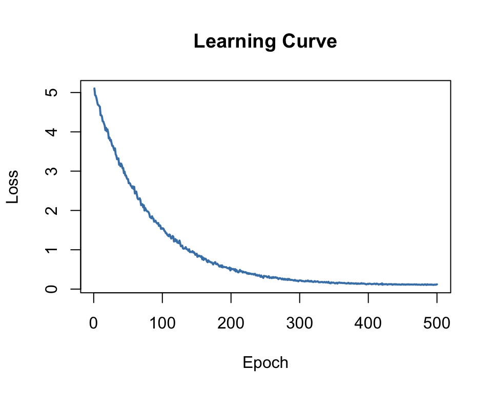
The Learning Curve

Plot loss vs epoch to monitor training:

learning_curve = []
for epoch in range(10000):
    ...
    learning_curve.append(loss.item())

qplot(range(10000), learning_curve,
      xlab="epoch", ylab="loss")

• Dropping = model is learning
• Flat = converged (or stuck)
• Increasing = learning rate too high!

Your Turn: Explore the Playground

Open playground.hakyimlab.org and try:

1. Regression → Cubic: increase neurons from 1 to 8 — watch the fit improve
2. Switch to Classification → Circle: same idea, different task
3. Set activation to Linear — can it ever fit a curve or separate a circle?
4. Crank learning rate to 1.0 — what happens to the loss?
5. Turn on “Show test data” — is a big network overfitting?

DNA as Data: One-Hot Encoding

How do we feed DNA to a neural network?

Sequence:  A  T  G  C  G  T  A

           A  T  G  C
     1:  [ 1  0  0  0 ]  ← A
     2:  [ 0  1  0  0 ]  ← T
     3:  [ 0  0  1  0 ]  ← G
     4:  [ 0  0  0  1 ]  ← C
     5:  [ 0  0  1  0 ]  ← G
     6:  [ 0  1  0  0 ]  ← T
     7:  [ 1  0  0  0 ]  ← A

Shape: (sequence_length, 4)

Each base → a 4-dimensional unit vector. No ordinal relationship imposed.

From DNA to Prediction

DNA sequence          One-hot matrix       Neural network      Prediction

ATGCGTAACG...  →  ┌─────────────┐   →   ┌──────────┐   →   binding score
                  │ 1 0 0 0     │       │  MLP or  │       expression level
                  │ 0 1 0 0     │       │   CNN    │       variant effect
                  │ 0 0 1 0     │       │          │       ...
                  │ 0 0 0 1     │       └──────────┘
                  │ ...         │
                  └─────────────┘

This is the core pattern of the most of the course.

Every model we study takes DNA sequence as input and predicts a biological output.

MLP vs CNN: A Preview

MLP (this unit)

• Flatten DNA → single vector
• Every input connected to every neuron
• No concept of “position”
• Good for learning the basics

CNN (next)

• Preserve sequential structure
• Sliding window = motif scanner
• Learned filters ≈ PWMs
• The workhorse of genomic DL

A CNN filter sliding over one-hot DNA is mathematically equivalent to scoring with a Position Weight Matrix (PWM) — but learned from data!

Unit 0 Plan: Weeks 1–3

Session	Topic	Notebook
Week 1a	Setup, intro	(this lecture)
Week 1b	Linear → MLP in PyTorch	hands-on-introduction_to_deep_learning.ipynb
Week 2	CNN for DNA scoring	updated-basic_DNA_tutorial.ipynb
Week 3a	TF binding project	tf-binding-prediction-starter.ipynb
Week 3b	Hyperparameter tuning	tf-binding-wandb.ipynb

What’s Coming Next

Unit 1: Transformers & GPT

• Attention mechanism
• Karpathy’s nanoGPT
• Train a DNA language model
• Fine-tune for promoter prediction

Unit 2: Enformer & Borzoi

• Predict epigenome from 200kb DNA
• Variant effect prediction
• Connection to GWAS/PrediXcan

The arc: MLP → CNN → Transformer → Genomic foundation models

Resources

Videos:

• 3Blue1Brown: Neural Networks — beautiful visual intuition
• Karpathy: Building GPT from scratch — we’ll use this in Unit 1

Interactive:

• playground.hakyimlab.org — experiment with MLP architecture interactively
• playground-guide.md — reference for all playground controls

Getting Started

Environment: Google Colab (GPU provided, no local setup needed)

First notebook: hands-on-introduction_to_deep_learning.ipynb

device = torch.device('cuda' if torch.cuda.is_available() else 'cpu')

Questions?